%matplotlib inline
from d2l import torch as d2l
import numpy as np
import torch
from torch import nn29.4 Score Matching, Diffusion, and Flow Matching
The preceding sections developed ODE solvers (Section 29.1), forward noising SDEs (Section 29.2), and the role of the score \(\nabla \log p_t\) in probability flow and time reversal (Section 29.3). This section studies how to estimate a score or velocity field by regression and then sample by integrating the resulting ODE or SDE. We develop score matching and its denoising form, interpret DDPM (Ho et al. 2020) as a discretized variance-preserving SDE, derive Langevin sampling, DDIM, and guidance from the same score calculus, and then develop flow matching and rectified flow as methods that prescribe a noise-to-data path, and relate straight paths to kinetic energy in optimal transport (Y. Song, Sohl-Dickstein, et al. 2021; Lipman et al. 2023).
The principal statistical device is conditional expectation. A marginal score or velocity may be unavailable directly but can be expressed as the conditional expectation of a tractable per-sample quantity. Least-squares regression against that quantity recovers its conditional mean. This identity supports both denoising score matching and conditional flow matching.
We lean on the Fokker–Planck equation and the probability-flow ODE (Section 29.3.2, Section 29.3.3.3), the Ornstein–Uhlenbeck process (Section 29.2.4), Euler and Euler–Maruyama steps (Section 29.1.3, Section 29.2.3.2), and the divergences of Section 28.2 (Fisher divergence via Section 28.2.4.1, optimal transport via Section 28.2.3.3). The numerical examples include two short training loops (a one-dimensional score network in NumPy and a two-dimensional flow-matching model, the latter retrained once more to measure reflow) plus closed-form simulations for the remaining examples.
%matplotlib inline
from d2l import tensorflow as d2l
import numpy as np
import tensorflow as tf%matplotlib inline
from d2l import jax as d2l
import jax
from jax import numpy as jnp
import numpy as np
import optax%matplotlib inline
from d2l import mxnet as d2l
from mxnet import autograd, gluon, init, npx
from mxnet import np as mxnp
import numpy as np
npx.set_np()29.4.1 Learning the Score
29.4.1.1 A Normalizer-Free Objective
Fitting a density \(p_{\boldsymbol{\theta}}\) to data by maximum likelihood requires evaluating its normalizing constant, which for a neural-network energy-based model is a \(d\)-dimensional integral with no closed form. The score \(\nabla_{\mathbf{x}} \log p_{\boldsymbol{\theta}}\) is independent of that constant (Equation 28.2.13; re-derived for energy-based models in Section 29.3.4). Objectives and samplers formulated only in terms of scores therefore need not evaluate that constant. Instead of matching densities, match score fields: take a model \(\mathbf{s}_{\boldsymbol{\theta}} : \mathbb{R}^d \to \mathbb{R}^d\) (any vector field, e.g. a neural network; it need not be a gradient) and minimize the Fisher divergence between model and data (Section 28.2.4.1),
\[ J_{\mathrm{ESM}}(\boldsymbol{\theta}) = \tfrac{1}{2}\, \mathbb{E}_{\mathbf{x} \sim p} \left[\, \left\| \mathbf{s}_{\boldsymbol{\theta}}(\mathbf{x}) - \nabla \log p(\mathbf{x}) \right\|^2 \right], \tag{29.4.1}\]
called explicit score matching. This removes the normalizer, but the objective still contains \(\nabla \log p\), the score of the data distribution, which is exactly what we do not know. Hyvärinen’s insight is that an integration by parts removes it (Hyvärinen 2005).
Proposition (Hyvärinen’s identity). Let \(p\) be a smooth positive density and \(\mathbf{s}_{\boldsymbol{\theta}}\) a smooth vector field, with \(p(\mathbf{x})\, \mathbf{s}_{\boldsymbol{\theta}}(\mathbf{x}) \to \mathbf{0}\) as \(\|\mathbf{x}\| \to \infty\) and all the expectations below finite. Then
\[ J_{\mathrm{ESM}}(\boldsymbol{\theta}) = \mathbb{E}_{\mathbf{x} \sim p} \left[\, \tfrac{1}{2} \| \mathbf{s}_{\boldsymbol{\theta}}(\mathbf{x}) \|^2 + \nabla \cdot \mathbf{s}_{\boldsymbol{\theta}}(\mathbf{x}) \right] + C, \tag{29.4.2}\]
where \(\nabla \cdot \mathbf{s}_{\boldsymbol{\theta}} = \sum_i \partial s_i / \partial x_i\) is the divergence and \(C\) does not depend on \(\boldsymbol{\theta}\).
Proof. Expand the square in Equation 29.4.1: the term \(\tfrac12 \mathbb{E}\|\nabla \log p\|^2\) is the constant \(C\), the term \(\tfrac12 \mathbb{E}\|\mathbf{s}_{\boldsymbol{\theta}}\|^2\) appears verbatim in Equation 29.4.2, and it remains to transform the cross term. In one dimension,
\[ -\mathbb{E}_{x \sim p}\left[ s_{\boldsymbol{\theta}}(x)\, (\log p)'(x) \right] = -\int s_{\boldsymbol{\theta}}(x)\, \frac{p'(x)}{p(x)}\, p(x)\, dx = -\int s_{\boldsymbol{\theta}}(x)\, p'(x)\, dx, \]
and integrating by parts with the boundary term \(\left[ s_{\boldsymbol{\theta}} \, p \right]_{-\infty}^{\infty} = 0\) leaves \(+\int s_{\boldsymbol{\theta}}'(x)\, p(x)\, dx = \mathbb{E}_p[s_{\boldsymbol{\theta}}']\). This step replaces the unknown score with a derivative of the model. In \(d\) dimensions, apply the same one-dimensional step to each coordinate \(i\) (with \(s_i\) in place of \(s_{\boldsymbol{\theta}}\) and \(\partial_i p\) in place of \(p'\), integrating coordinate-wise, which Fubini justifies under the stated integrability) and sum: the cross term becomes \(\mathbb{E}_p[\sum_i \partial_i s_i] = \mathbb{E}_p[\nabla \cdot \mathbf{s}_{\boldsymbol{\theta}}]\). \(\blacksquare\)
Every quantity in Equation 29.4.2 is an expectation under \(p\) of something we can evaluate, so we can minimize it from samples alone, with no \(Z_{\boldsymbol{\theta}}\) and no \(\nabla \log p\); the right-hand side is called implicit score matching. The two terms have complementary effects. The \(\nabla \cdot \mathbf{s}_{\boldsymbol{\theta}}\) term favors score fields with negative divergence at the samples, as for \(-\nabla E\) near a minimum, while \(\tfrac12\|\mathbf{s}_{\boldsymbol{\theta}}\|^2\) penalizes fields of unbounded magnitude.
Implicit score matching is expensive in high dimensions. The divergence is the trace of the Jacobian, \(\nabla \cdot \mathbf{s}_{\boldsymbol{\theta}} = \operatorname{tr}\, (\partial \mathbf{s}_{\boldsymbol{\theta}} / \partial \mathbf{x})\), and computing it exactly generally requires derivative work that scales linearly with \(d\) (for example, one reverse-mode pass per Jacobian row) (Section 25.3): the same trace bottleneck that afflicts continuous normalizing flows (Section 29.1.5), and just as there, Hutchinson trace estimates only trade compute for variance. For images, \(d\) is in the millions. Denoising score matching avoids this trace computation.
29.4.1.2 Denoising Score Matching
Score models become practical by matching the score of Gaussian-blurred data rather than the clean data distribution (Vincent 2011). Perturb each sample with Gaussian noise of scale \(\sigma\):
\[ \tilde{\mathbf{x}} = \mathbf{x} + \sigma \boldsymbol{\epsilon}, \qquad \boldsymbol{\epsilon} \sim \mathcal{N}(\mathbf{0}, I), \qquad \textrm{i.e.}\quad p_\sigma(\tilde{\mathbf{x}} \mid \mathbf{x}) = \mathcal{N}(\tilde{\mathbf{x}};\, \mathbf{x},\, \sigma^2 I). \]
The noised marginal \(p_\sigma(\tilde{\mathbf{x}}) = \int p_\sigma(\tilde{\mathbf{x}} \mid \mathbf{x})\, p(\mathbf{x})\, d\mathbf{x}\) is the data density convolved with a Gaussian and approaches \(p\) as \(\sigma\) decreases. Its score is still intractable, but the score of the conditional follows directly by taking \(\log\) of the Gaussian density:
\[ \nabla_{\tilde{\mathbf{x}}} \log p_\sigma(\tilde{\mathbf{x}} \mid \mathbf{x}) = \frac{\mathbf{x} - \tilde{\mathbf{x}}}{\sigma^2} = -\frac{\boldsymbol{\epsilon}}{\sigma}. \tag{29.4.3}\]
This vector points from the noisy observation toward the corresponding clean sample. Denoising score matching (DSM) uses it as a regression target:
\[ J_{\mathrm{DSM}}(\boldsymbol{\theta}) = \mathbb{E}_{\mathbf{x} \sim p,\ \tilde{\mathbf{x}} \sim p_\sigma(\cdot \mid \mathbf{x})} \left[\, \left\| \mathbf{s}_{\boldsymbol{\theta}}(\tilde{\mathbf{x}}) - \nabla_{\tilde{\mathbf{x}}} \log p_\sigma(\tilde{\mathbf{x}} \mid \mathbf{x}) \right\|^2 \right]. \tag{29.4.4}\]
The regression target depends on the sampled clean point, whereas the desired score depends only on the noisy observation. Least squares connects them by fitting the target’s conditional mean. The following lemma states that fact; the flow-matching argument will use it again with a velocity target.
Lemma (regression to the conditional mean). Let \((X, Y)\) be jointly distributed with \(\mathbb{E}\|Y\|^2 < \infty\) and let \(\mathbf{m}(X) = \mathbb{E}[Y \mid X]\). Then for every measurable \(\mathbf{v}\),
\[ \mathbb{E} \left\| \mathbf{v}(X) - Y \right\|^2 = \mathbb{E} \left\| \mathbf{v}(X) - \mathbf{m}(X) \right\|^2 + \mathbb{E} \left\| Y - \mathbf{m}(X) \right\|^2. \tag{29.4.5}\]
The second term does not involve \(\mathbf{v}\): minimizing a least-squares loss against the noisy target \(Y\) is the same problem as minimizing it against the conditional mean \(\mathbf{m}(X)\), up to an additive constant.
Proof. Insert \(\pm\mathbf{m}(X)\) and expand. The cross term is \(2\, \mathbb{E}\left[ (\mathbf{v}(X) - \mathbf{m}(X))^\top (\mathbf{m}(X) - Y) \right]\); conditioning on \(X\) (the tower rule, Section 27.1) and using \(\mathbb{E}[\mathbf{m}(X) - Y \mid X] = \mathbf{0}\) makes it vanish. \(\blacksquare\)
Proposition (Vincent’s theorem). Under the conditions above, with expectations finite,
\[ J_{\mathrm{DSM}}(\boldsymbol{\theta}) = \mathbb{E}_{\tilde{\mathbf{x}} \sim p_\sigma} \left[\, \left\| \mathbf{s}_{\boldsymbol{\theta}}(\tilde{\mathbf{x}}) - \nabla \log p_\sigma(\tilde{\mathbf{x}}) \right\|^2 \right] + C, \]
with \(C\) independent of \(\boldsymbol{\theta}\): denoising score matching and explicit score matching on the noised marginal (the right-hand side is twice Equation 29.4.1 with \(p_\sigma\) in place of \(p\)) have the same minimizers and, up to that overall factor of two, the same gradients.
Proof. Apply the lemma with \(X = \tilde{\mathbf{x}}\) and \(Y = \nabla_{\tilde{\mathbf{x}}} \log p_\sigma(\tilde{\mathbf{x}} \mid \mathbf{x})\). It remains to identify the conditional mean, and the marginal score is the posterior mean of the conditional scores:
\[ \mathbb{E}\left[ Y \mid \tilde{\mathbf{x}} \right] = \int \frac{\nabla_{\tilde{\mathbf{x}}}\, p_\sigma(\tilde{\mathbf{x}} \mid \mathbf{x})}{p_\sigma(\tilde{\mathbf{x}} \mid \mathbf{x})} \; \frac{p_\sigma(\tilde{\mathbf{x}} \mid \mathbf{x})\, p(\mathbf{x})}{p_\sigma(\tilde{\mathbf{x}})}\, d\mathbf{x} = \frac{\nabla_{\tilde{\mathbf{x}}} \int p_\sigma(\tilde{\mathbf{x}} \mid \mathbf{x})\, p(\mathbf{x})\, d\mathbf{x}}{p_\sigma(\tilde{\mathbf{x}})} = \nabla \log p_\sigma(\tilde{\mathbf{x}}), \]
where the first equality writes out the posterior \(p(\mathbf{x} \mid \tilde{\mathbf{x}})\) by Bayes’ rule and the second swaps the gradient with the integral. \(\blacksquare\)
The proof does not require a Gaussian kernel: any smooth noising kernel satisfying the stated conditions works. Gaussian noise is convenient because its conditional score Equation 29.4.3 is linear in the noise. By Equation 29.4.3, predicting the score and predicting the noise \(\boldsymbol{\epsilon}\) differ only by the factor \(-1/\sigma\); this is the \(\boldsymbol{\epsilon}\)-prediction parameterization used in diffusion models. Two corollaries follow.
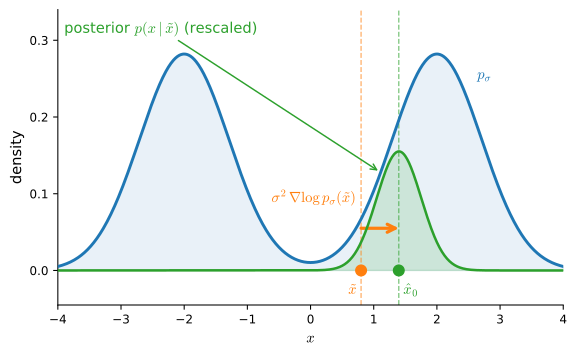
- Tweedie’s formula (Efron 2011). Rearranging \(\mathbb{E}[(\mathbf{x} - \tilde{\mathbf{x}})/\sigma^2 \mid \tilde{\mathbf{x}}] = \nabla \log p_\sigma(\tilde{\mathbf{x}})\) gives \(\mathbb{E}[\mathbf{x} \mid \tilde{\mathbf{x}}] = \tilde{\mathbf{x}} + \sigma^2\, \nabla \log p_\sigma(\tilde{\mathbf{x}})\): the optimal denoiser adds a score-based correction (Figure 29.4.1). Under squared error and Gaussian corruption, the posterior-mean denoiser is determined by the marginal score.
- The population loss need not go to zero. By Equation 29.4.5, the DSM loss at the optimum equals \(\mathbb{E}\|Y - \mathbf{m}(X)\|^2\), the average posterior variance of the conditional score: many clean points \(\mathbf{x}\) explain the same \(\tilde{\mathbf{x}}\), and no network can resolve which one produced it. A resulting Bayes risk depends on the noise level, weighting, and target parameterization. An observed training loss also contains approximation and optimization error, so it should be compared with an estimated Bayes-risk floor rather than with zero.
29.4.1.3 A Score Network in One Dimension
Take the bimodal mixture \(p = \tfrac12 \mathcal{N}(-2, 0.5^2) + \tfrac12 \mathcal{N}(2, 0.5^2)\), noise scale \(\sigma = 0.5\), and fit a tiny multilayer perceptron \(s_{\boldsymbol{\theta}} : \mathbb{R} \to \mathbb{R}\) by minimizing Equation 29.4.4: the inputs are noised samples, the regression targets are \(-\epsilon/\sigma\), and training requires samples rather than an analytic expression for the true density. Because the noised marginal is again a Gaussian mixture (variance \(0.5^2 + \sigma^2 = 0.5\) per component), we have the analytic \(\nabla \log p_\sigma\) against which to evaluate the result. The network is small enough that we write its forward pass, its backward pass (Section 25.3), and an Adam update directly in plain NumPy, without an automatic-differentiation framework.
rng = np.random.default_rng(7)
n, sigma = 4096, 0.5
x = rng.normal(4.0 * rng.integers(0, 2, n) - 2.0, 0.5)    # x ~ p, the mixture

def mixture_score(q, var, means=(-2.0, 2.0)):             # analytic score
    w = np.stack([np.exp(-(q - m)**2 / (2 * var)) for m in means])
    return (w * np.stack([(m - q) / var for m in means])).sum(0) / w.sum(0)

# A 1 -> 32 -> 1 tanh network, with hand-written backprop and Adam updates
W1, b1 = rng.normal(size=(1, 32)), np.zeros(32)
W2, b2 = rng.normal(size=(32, 1)) / np.sqrt(32), np.zeros(1)
params = [W1, b1, W2, b2]
mom = [np.zeros_like(p) for p in params]
vel = [np.zeros_like(p) for p in params]
for step in range(2000):
    eps = rng.standard_normal(n)                          # fresh noise per step
    xt, y = (x + sigma * eps)[:, None], (-eps / sigma)[:, None]
    H = np.tanh(xt @ W1 + b1)                             # forward pass
    S = H @ W2 + b2
    G = 2 * (S - y) / n                                   # backward pass
    GH = (G @ W2.T) * (1 - H**2)
    grads = [xt.T @ GH, GH.sum(0), H.T @ G, G.sum(0)]
    for p, g, m, v in zip(params, grads, mom, vel):       # Adam updates
        m[:] = 0.9 * m + 0.1 * g
        v[:] = 0.999 * v + 0.001 * g * g
        p -= 1e-2 * m / (np.sqrt(v) + 1e-8)
loss = ((S - y)**2).mean()
bayes_ref = ((mixture_score(x + sigma * eps, 0.5) + eps / sigma)**2).mean()
grid = np.linspace(-4, 4, 201)
s_hat = (np.tanh(grid[:, None] @ W1 + b1) @ W2 + b2)[:, 0]
print(f'DSM loss {loss:.3f} vs estimated Bayes risk {bayes_ref:.3f}; '
      f'max |s_theta - score| on [-4, 4]: {np.abs(s_hat - mixture_score(grid, 0.5)).max():.3f}')
d2l.plot(grid, [mixture_score(grid, 0.5), s_hat], 'x', 'score',
legend=['analytic score of p_sigma', 'learned s_theta'])DSM loss 2.036 vs estimated Bayes risk 2.038; max |s_theta - score| on [-4, 4]: 0.199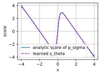
DSM loss 2.036 vs estimated Bayes risk 2.038; max |s_theta - score| on [-4, 4]: 0.199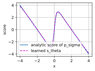
DSM loss 2.036 vs estimated Bayes risk 2.038; max |s_theta - score| on [-4, 4]: 0.199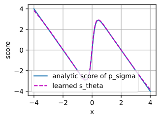
DSM loss 2.036 vs estimated Bayes risk 2.038; max |s_theta - score| on [-4, 4]: 0.199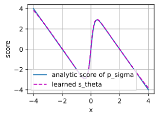
The learned field tracks the analytic score across both modes and the low-density valley between them: the largest gap on \([-4, 4]\) is about \(0.2\), on a curve whose values span \(\pm 4\) (the smoothed score is \(s(x) = 4\tanh(4x) - 2x\), extremal at the interval ends). And the printout verifies the regression lemma numerically: the final DSM loss (\(\approx 2.04\)) is close to the estimated Bayes risk \(\mathbb{E}\|Y - \mathbf{m}(X)\|^2\) (\(\approx 2.04\), estimated on this finite sample with the analytic score). Their agreement is consistent with little reducible error remaining in this particular fit.
29.4.2 Score-Based Diffusion Models
29.4.2.1 Scores Across Noise Levels
A single noise scale \(\sigma\) creates a trade-off. Small \(\sigma\) makes \(p_\sigma \approx p\), but noised samples then seldom enter low-density regions, so the learned score is poorly constrained where a sampler initialized from random noise may need it. Large \(\sigma\) provides broader coverage but estimates the score of an over-smoothed density. The standard solution (Song and Ermon 2019; Y. Song, Sohl-Dickstein, et al. 2021): learn the score at every noise level along a forward process that moves the data toward a tractable reference, by making the network noise-conditional, \(\mathbf{s}_{\boldsymbol{\theta}}(\mathbf{x}, t)\) (Figure 29.4.2, the two-dimensional companion of the one-dimensional density movie in Figure 29.3.4). Section 29.2 gave us the two standard forward processes:
- the variance-exploding (VE) SDE \(d\mathbf{X} = \sqrt{\tfrac{d}{dt}\sigma^2(t)}\; d\mathbf{W}\), with \(\sigma^2(t)\) increasing and differentiable so that the square root exists, which adds noise without shrinking the data: \(\mathbf{x}_t = \mathbf{x}_0 + \sigma(t) \boldsymbol{\epsilon}\) (the continuous limit of Song & Ermon’s noise ladder), with conditional terminal law \(\mathcal{N}(\mathbf{x}_0, \sigma_{\max}^2 I)\) rather than a standard Gaussian;
- the variance-preserving (VP) SDE \(d\mathbf{X} = -\tfrac12 \beta(t)\, \mathbf{X}\, dt + \sqrt{\beta(t)}\; d\mathbf{W}\) of Equation 29.2.16, an Ornstein–Uhlenbeck process with a time-dependent rate (Section 29.2.4), which shrinks the signal as it adds noise so that unit-variance data keeps unit variance for all \(t\) (shown for the discrete chain below).
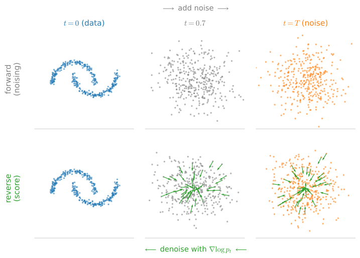
In both cases the transition kernel \(p_t(\mathbf{x}_t \mid \mathbf{x}_0)\) is an explicit Gaussian, so the DSM machinery applies verbatim at every \(t\): the training loss is the noise-conditional DSM objective
\[ \mathcal{L}(\boldsymbol{\theta}) = \mathbb{E}_{t}\, \lambda(t)\; \mathbb{E}_{\mathbf{x}_0,\, \mathbf{x}_t \sim p_t(\cdot \mid \mathbf{x}_0)} \left[\, \left\| \mathbf{s}_{\boldsymbol{\theta}}(\mathbf{x}_t, t) - \nabla_{\mathbf{x}_t} \log p_t(\mathbf{x}_t \mid \mathbf{x}_0) \right\|^2 \right], \tag{29.4.6}\]
with a weighting \(\lambda(t) > 0\) that decides which noise levels the network should serve best. In the population problem, with an unrestricted function class and positive weight at \(t\), Vincent’s theorem makes the minimizer \(\mathbf{s}(\cdot,t)=\nabla\log p_t\). A finite network trained on samples adds approximation, estimation, and optimization error. With the likelihood weighting \(\lambda(t)=g(t)^2\), the cited analysis relates the population score loss to an upper bound on negative log-likelihood under its regularity and terminal-distribution assumptions (Y. Song, Durkan, et al. 2021). DDPM’s simple loss instead induces \(\lambda(t)=1-\bar{\alpha}_t\), derived below; this changes the relative emphasis across noise levels and is often chosen for sample quality rather than for that bound. Generation then follows the program of Section 29.3.5 and Section 29.3.3.3: start from the chosen terminal reference (approximately Gaussian at finite noising time) and integrate either the reverse-time SDE (Anderson 1982) or the probability-flow ODE, with \(\mathbf{s}_{\boldsymbol{\theta}}\) standing in for the true score. A generative model is specified by this combination of forward process, learned score, and numerical sampler.
ImportantTwo clocks: the time conventions of diffusion and flow matching
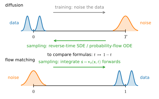
The two literatures run time in opposite directions, and almost every sign confusion in this field traces back to it (Figure 29.4.3).
- Diffusion noises data into noise forward in time: \(t = 0\) is data, \(t = T\) is (approximately) pure Gaussian. Sampling integrates backwards, from \(t = T\) down to \(0\).
- Flow matching parameterizes the generative direction: \(t = 0\) is noise, \(t = 1\) is data, and sampling integrates forwards from \(0\) to \(1\).
In this section, \(t\) in a diffusion formula runs data \(\to\) noise, and \(t\) in a flow-matching formula runs noise \(\to\) data. When comparing the two (as the unifying table at the end does), substitute \(t \mapsto 1 - t\) in one of them.
29.4.2.2 DDPM as a Discretized SDE
The Denoising Diffusion Probabilistic Model (Ho et al. 2020) looks, at first sight, like a different theory: a discrete-time Markov chain of \(T\) noising steps with schedule \(\beta_1, \ldots, \beta_T \in (0, 1)\),
\[ \mathbf{x}_t = \sqrt{1 - \beta_t}\; \mathbf{x}_{t-1} + \sqrt{\beta_t}\; \boldsymbol{\epsilon}_t, \qquad \boldsymbol{\epsilon}_t \sim \mathcal{N}(\mathbf{0}, I)\ \textrm{i.i.d.} \tag{29.4.7}\]
It is not a different theory. Three short propositions identify it, piece by piece, with the VP picture above.
Proposition (the DDPM step is Euler–Maruyama on the VP-SDE). Discretize the VP-SDE with step \(\Delta\) and write \(\beta_t = \beta(t\Delta)\, \Delta\). The Euler–Maruyama step (Section 29.2.3.2) is
\[ \mathbf{x}_t = \left(1 - \tfrac{1}{2} \beta_t\right) \mathbf{x}_{t-1} + \sqrt{\beta_t}\; \boldsymbol{\epsilon}_t, \]
which agrees with the DDPM step Equation 29.4.7 to first order in \(\beta_t\).
Proof. The Taylor expansion \(\sqrt{1 - \beta} = 1 - \tfrac12 \beta - \tfrac18 \beta^2 - \cdots\) shows the two coefficients differ by \(O(\beta_t^2)\), while the noise terms are identical. \(\blacksquare\)
The agreement is first-order only (for the largest practical \(\beta_t \approx 0.02\) the coefficients differ in the fifth decimal), but DDPM’s exact form is in one way nicer than the discretization that inspired it: it has an exact closed-form marginal, with no \(O(\beta^2)\) apology.
Proposition (the \(\bar{\alpha}\)-marginal). Let \(\alpha_t = 1 - \beta_t\) and \(\bar{\alpha}_t = \prod_{s=1}^{t} \alpha_s\). Then conditionally on \(\mathbf{x}_0\),
\[ \mathbf{x}_t = \sqrt{\bar{\alpha}_t}\; \mathbf{x}_0 + \sqrt{1 - \bar{\alpha}_t}\; \boldsymbol{\epsilon}, \qquad \boldsymbol{\epsilon} \sim \mathcal{N}(\mathbf{0}, I). \tag{29.4.8}\]
Proof. Induction on \(t\); the case \(t = 0\) is trivial. Assume Equation 29.4.8 at \(t - 1\) and substitute into Equation 29.4.7:
\[ \mathbf{x}_t = \sqrt{\alpha_t \bar{\alpha}_{t-1}}\; \mathbf{x}_0 + \sqrt{\alpha_t (1 - \bar{\alpha}_{t-1})}\; \bar{\boldsymbol{\epsilon}} + \sqrt{\beta_t}\; \boldsymbol{\epsilon}_t, \]
with \(\bar{\boldsymbol{\epsilon}}, \boldsymbol{\epsilon}_t\) independent standard Gaussians. A sum of independent Gaussians is Gaussian with summed variances: \(\alpha_t (1 - \bar{\alpha}_{t-1}) + \beta_t = \alpha_t - \bar{\alpha}_t + 1 - \alpha_t = 1 - \bar{\alpha}_t\), and \(\alpha_t \bar{\alpha}_{t-1} = \bar{\alpha}_t\). \(\blacksquare\)
The term “variance-preserving” follows from the identity: for unit-variance data, \(\mathrm{Var}(\mathbf{x}_t) = \bar{\alpha}_t \cdot 1 + (1 - \bar{\alpha}_t) = 1\) for every \(t\), not merely in the limit. And because Equation 29.4.8 is a Gaussian kernel with scale \(\sqrt{1 - \bar{\alpha}_t}\), denoising score matching applies directly.
Proposition (the DDPM loss is reweighted DSM). The conditional score of Equation 29.4.8 is \(\nabla_{\mathbf{x}_t} \log p(\mathbf{x}_t \mid \mathbf{x}_0) = -\boldsymbol{\epsilon} / \sqrt{1 - \bar{\alpha}_t}\). Hence, parameterizing the score model through a noise-prediction network, \(\mathbf{s}_{\boldsymbol{\theta}}(\mathbf{x}_t, t) = -\boldsymbol{\epsilon}_{\boldsymbol{\theta}}(\mathbf{x}_t, t) / \sqrt{1 - \bar{\alpha}_t}\), the DDPM “simple loss” \(\mathbb{E}_{t, \mathbf{x}_0, \boldsymbol{\epsilon}} \| \boldsymbol{\epsilon} - \boldsymbol{\epsilon}_{\boldsymbol{\theta}}(\mathbf{x}_t, t) \|^2\) equals the noise-conditional DSM loss Equation 29.4.6 with weighting \(\lambda(t) = 1 - \bar{\alpha}_t\).
Proof. Differentiate \(\log p(\mathbf{x}_t \mid \mathbf{x}_0) = -\|\mathbf{x}_t - \sqrt{\bar{\alpha}_t} \mathbf{x}_0\|^2 / (2 (1 - \bar{\alpha}_t)) + \textrm{const}\) and substitute Equation 29.4.8. Then
\[ \left\| \mathbf{s}_{\boldsymbol{\theta}}(\mathbf{x}_t, t) + \frac{\boldsymbol{\epsilon}}{\sqrt{1 - \bar{\alpha}_t}} \right\|^2 = \frac{1}{1 - \bar{\alpha}_t} \left\| \boldsymbol{\epsilon} - \boldsymbol{\epsilon}_{\boldsymbol{\theta}}(\mathbf{x}_t, t) \right\|^2, \]
so the two losses differ exactly by the factor \(\lambda(t) = 1 - \bar{\alpha}_t\) inside the time expectation. \(\blacksquare\)
So DDPM = VP forward process + DSM objective in \(\boldsymbol{\epsilon}\)-parameterization + ancestral sampling, i.e. stepping through the learned reverse chain one noise level at a time. The discrete chain is a first-order counterpart of the continuous VP construction (Y. Song, Sohl-Dickstein, et al. 2021). Historically the model was derived along an entirely different route: write the reverse chain as a latent-variable model and maximize an evidence lower bound, as in Section 27.3.5. After the same Gaussian algebra as above, the KL terms between the Gaussian forward posteriors and the learned reverse steps collapse into weighted \(\boldsymbol{\epsilon}\)-prediction losses; the ELBO and score-based derivations produce the same objective with a different \(\lambda(t)\), and Luo (2022) is a careful walkthrough of that equivalence.
The cell below checks both propositions at once: it runs the discrete chain Equation 29.4.7 for \(T = 1000\) steps on (standardized) samples of our two-Gaussian mixture and compares against the closed form Equation 29.4.8: variances on the way, and the full distribution against a one-shot \(\bar{\alpha}\)-sample at the end.
rng = np.random.default_rng(13)
T = 1000
beta = np.linspace(1e-4, 0.02, T)                  # the DDPM schedule
alpha_bar = np.cumprod(1.0 - beta)
x0 = x / x.std()                                   # unit-variance mixture data
xt = x0.copy()
for t in range(T):                                 # the discrete forward chain
    xt = np.sqrt(1 - beta[t]) * xt + np.sqrt(beta[t]) * rng.standard_normal(n)
    if t + 1 in (10, 100, 1000):
        var_pred = alpha_bar[t] * x0.var() + (1 - alpha_bar[t])
        print(f't = {t+1:4d}: Var(x_t) chain {xt.var():.3f}, '
              f'formula {var_pred:.3f}, alpha_bar {alpha_bar[t]:.4f}')
one_shot = (np.sqrt(alpha_bar[-1]) * x0
            + np.sqrt(1 - alpha_bar[-1]) * rng.standard_normal(n))
print(f'chain vs one-shot at T: mean {xt.mean():+.3f} vs {one_shot.mean():+.3f}, '
      f'std {xt.std():.3f} vs {one_shot.std():.3f}')
t = 10: Var(x_t) chain 1.000, formula 1.000, alpha_bar 0.9981
t = 100: Var(x_t) chain 0.994, formula 1.000, alpha_bar 0.8970
t = 1000: Var(x_t) chain 1.024, formula 1.000, alpha_bar 0.0000
chain vs one-shot at T: mean -0.027 vs +0.005, std 1.012 vs 1.000The variance tracks the formula’s \(1.000\) at every checkpoint, to within the sampling error of a \(4096\)-point variance estimate (the VP identity in action), and after a thousand steps the chain matches the one-shot Gaussian reparameterization in distribution, which is why DDPM training never simulates the chain: it jumps straight to any \(t\) via Equation 29.4.8.
29.4.2.3 Langevin Dynamics and Predictor–Corrector Sampling
Reverse-time SDEs are not the only way to turn a score into samples: the oldest way predates diffusion models by decades. Suppose we hold the distribution fixed: no noising schedule, just a target \(p\) whose score we know. Langevin dynamics is the SDE whose drift pushes up the log-density while noise jiggles the state,
\[ d\mathbf{X} = \tfrac{1}{2} \nabla \log p(\mathbf{X})\, dt + d\mathbf{W}. \tag{29.4.9}\]
Proposition (stationarity). Let \(p\) be a smooth positive density with \(p\) and \(\nabla p\) vanishing at infinity. Then \(p\) is a stationary density of Equation 29.4.9: if \(\mathbf{X}_0 \sim p\) then \(\mathbf{X}_t \sim p\) for all \(t \ge 0\).
Proof. The Fokker–Planck equation (Section 29.3.2) for drift \(\mathbf{b} = \tfrac12 \nabla \log p\) and unit diffusion reads \(\partial_t \rho = -\nabla \cdot (\rho\, \mathbf{b}) + \tfrac12 \Delta \rho\). Substitute \(\rho = p\) and use the identity \(p\, \nabla \log p = \nabla p\):
\[ -\nabla \cdot \left( \tfrac{1}{2}\, p\, \nabla \log p \right) + \tfrac{1}{2} \Delta p = -\tfrac{1}{2} \nabla \cdot (\nabla p) + \tfrac{1}{2} \Delta p = 0. \]
The right-hand side of the Fokker–Planck equation vanishes identically, so \(\rho \equiv p\) solves it for all time. \(\blacksquare\)
Discretizing Equation 29.4.9 by Euler–Maruyama with step \(h\) gives the Langevin sampler \(\mathbf{x} \leftarrow \mathbf{x} + \tfrac{h}{2}\, \mathbf{s}(\mathbf{x}) + \sqrt{h}\, \boldsymbol{\xi}\). Stationarity of the SDE is not convergence of its discretization. Under appropriate ergodicity and regularity assumptions, the finite-step chain has an invariant law that approximates \(p\), generally with \(O(h)\) weak bias (see Exercise 6); convergence to that law can still be slow. With \(\mathbf{s} = \mathbf{s}_{\boldsymbol{\theta}}\), this turns a trained score network directly into a generator. The cell runs it on our mixture with the analytic score, exposing that weakness along the way.
rng = np.random.default_rng(11)

def langevin(q, h, steps, rng):
    for _ in range(steps):
        q = q + 0.5 * h * mixture_score(q, 0.25) \
            + np.sqrt(h) * rng.standard_normal(q.shape)
    return q

warm = langevin(rng.normal(0.0, 3.0, 10000), 0.01, 2000, rng)
print(f'spread-out start: P(X > 0) = {(warm > 0).mean():.3f}, '
      f'E[X^2] = {(warm**2).mean():.2f} (truth 0.500, 4.25)')
cold = langevin(np.full(10000, -2.0), 0.01, 2000, rng)
print(f'one-mode start:   P(X > 0) = {(cold > 0).mean():.3f}  (slow mixing)')
spread-out start: P(X > 0) = 0.509, E[X^2] = 4.26 (truth 0.500, 4.25)
one-mode start: P(X > 0) = 0.012 (slow mixing)From a broad initial distribution, the chains approach the target proportions: half the mass lies in each mode, and the second moment matches the true value. When all chains start in the left mode, almost none cross after two thousand steps because the density between the modes is small and the score points back toward the current mode. This slow mixing makes plain Langevin sampling inefficient on multimodal targets and motivates the noise schedules used by diffusion models: annealed Langevin dynamics (Song and Ermon 2019) runs Langevin at a ladder of noise levels \(\sigma_1 > \cdots > \sigma_L\), using \(\mathbf{s}_{\boldsymbol{\theta}}(\cdot, \sigma_i)\) at level \(i\). At large \(\sigma\) the smoothed density has no barriers, so chains move between regions; as \(\sigma\) shrinks, detail re-emerges with the global proportions already right. The same idea survives inside modern samplers as the predictor–corrector scheme (Y. Song, Sohl-Dickstein, et al. 2021): alternate a reverse-SDE step (the predictor, which moves to the next noise level) with a few Langevin steps at the current level (the corrector, which repairs the discretization error of the predictor before it compounds).
29.4.2.4 DDIM: Trading Noise for Speed
Ancestral DDPM sampling needs \(T \sim 1000\) network calls. DDIM (Denoising Diffusion Implicit Models) (J. Song et al. 2021) cuts this by an order of magnitude with the same trained network (no retraining) by replacing the noisy reverse chain with a deterministic update.
NoteThe DDIM update, in one derivation
At time \(t\), the network’s noise prediction yields a current best guess of the clean sample by inverting the marginal Equation 29.4.8:
\[ \hat{\mathbf{x}}_0 = \frac{\mathbf{x}_t - \sqrt{1 - \bar{\alpha}_t}\; \boldsymbol{\epsilon}_{\boldsymbol{\theta}}(\mathbf{x}_t, t)}{\sqrt{\bar{\alpha}_t}}. \]
DDPM would resample by drawing fresh noise and forming a noisy \(\mathbf{x}_{t-1}\). DDIM instead reuses the predicted direction, forming \(\mathbf{x}_{t-1}\) from the current clean estimate \(\hat{\mathbf{x}}_0\) and noise estimate \(\boldsymbol{\epsilon}_{\boldsymbol{\theta}}\) at time \(t-1\):
\[ \mathbf{x}_{t-1} = \sqrt{\bar{\alpha}_{t-1}}\; \hat{\mathbf{x}}_0 + \sqrt{1 - \bar{\alpha}_{t-1}}\; \boldsymbol{\epsilon}_{\boldsymbol{\theta}}(\mathbf{x}_t, t). \tag{29.4.10}\]
The algebra is easiest to remember through a hypothetical forward pair: if we knew that realization’s actual \((\mathbf{x}_0,\boldsymbol{\epsilon})\), the formula would move it along the curve \(t \mapsto \sqrt{\bar{\alpha}_t}\,\mathbf{x}_0 + \sqrt{1-\bar{\alpha}_t}\,\boldsymbol{\epsilon}\). A network trained by squared error does not recover that latent noise realization, however; it recovers the conditional mean \(\mathbb{E}[\boldsymbol{\epsilon}\mid\mathbf{x}_t]\). Thus Equation 29.4.10 is a deterministic update defined from the learned conditional estimate, not an exact jump along each sample’s hidden forward curve. We may evaluate it on a sparse subsequence of the training noise levels, but larger gaps introduce discretization/model error.
Two remarks complete the picture. First, DDIM is the \(\eta = 0\) endpoint of a family that interpolates to an ancestral sampler by reinjecting noise; its non-Markovian forward construction has the same one-time noising marginals as DDPM, so the same trained network can be reused. Second, in the fine-step continuous-time limit the deterministic trajectory is related to the probability-flow ODE of the VP-SDE (Section 29.3.3.3). This relationship motivates sparse deterministic sampling, but it does not make a finite DDIM stride exact, even when a marginal happens to be Gaussian.
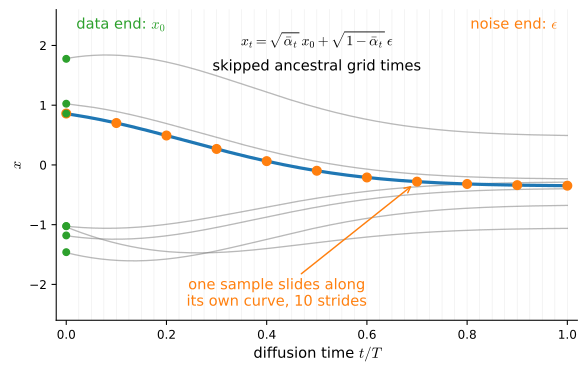
How much do the strides cost when the marginal is not a single Gaussian? Our standardized two-Gaussian mixture answers in closed form: its noised marginals, hence the exact noise prediction \(\boldsymbol{\epsilon}_{\boldsymbol{\theta}} = -\sqrt{1 - \bar{\alpha}_t}\; \nabla \log p_t\), are available at every \(t\), so we can run the DDIM update Equation 29.4.10 with no learning in the loop: a thousand small steps versus ten big ones from the same initial noise draws.
rng = np.random.default_rng(19)
mt, vt = 2 / np.sqrt(4.25), 0.25 / 4.25       # standardized mixture parameters

def ddim(z, K):                               # K deterministic DDIM strides
    idx = np.linspace(999, 0, K + 1).round().astype(int)
    xt = z.copy()
    for t1, t2 in zip(idx[:-1], idx[1:]):
        a1, a2 = alpha_bar[t1], alpha_bar[t2]
        s = mixture_score(xt, a1 * vt + 1 - a1,
                          (-np.sqrt(a1) * mt, np.sqrt(a1) * mt))
        eps = -np.sqrt(1 - a1) * s            # exact noise prediction
        x0_hat = (xt - np.sqrt(1 - a1) * eps) / np.sqrt(a1)
        xt = np.sqrt(a2) * x0_hat + np.sqrt(1 - a2) * eps
    return xt

def ks(a, b):                                 # two-sample KS statistic
    q = np.sort(np.concatenate([a, b]))
    return np.abs(np.searchsorted(np.sort(a), q, 'right') / len(a)
                  - np.searchsorted(np.sort(b), q, 'right') / len(b)).max()

z = rng.standard_normal(8000)
x_ref = ddim(z, 1000)                         # a thousand small staggers
for K in (10, 50):
    xK = ddim(z, K)
    print(f'{K:3d} strides vs 1000: mean |gap| {np.abs(xK - x_ref).mean():.3f}, '
          f'KS {ks(xK, x_ref):.3f}, mode fraction {(xK > 0).mean():.3f}')
print(f'mode fraction at 1000 steps: {(x_ref > 0).mean():.3f}; '
      'the same initial draws are used at every stride count')
10 strides vs 1000: mean |gap| 0.083, KS 0.080, mode fraction 0.495
50 strides vs 1000: mean |gap| 0.015, KS 0.018, mode fraction 0.495
mode fraction at 1000 steps: 0.495; the same initial draws are used at every stride countTen strides place every sample in the same mode as the thousand-step reference and differ by only \(0.08\) per sample on a scale where the modes sit at \(\pm 0.97\). (The mode fraction is identical at every stride count: the update is deterministic, and in this run no trajectory crosses the valley.) The discrepancy illustrates the central point: the predicted noise is a posterior mean, not the realization’s latent noise, so a finite deterministic stride need not preserve the target marginal exactly. This is true even for Gaussian data; Gaussianity makes the score linear, but does not turn the conditional mean into the sampled noise realization. By fifty strides the empirical CDF gap to the thousand-step numerical reference is \(0.018\). Since both runs use the same initial draws, this is a paired numerical comparison rather than an independent-sample hypothesis test. Larger strides reduce the number of evaluations while increasing finite-stride approximation error.
29.4.2.5 Guidance with Bayes’ Rule
Generative models often condition on a label or prompt. Conditioning a score model follows directly from probability identities and requires no new training objective. Bayes’ rule at noise level \(t\) reads \(p_t(\mathbf{x} \mid y) \propto p_t(\mathbf{x})\, p_t(y \mid \mathbf{x})\), and it becomes additive for scores, since the gradient is in \(\mathbf{x}\) and the evidence term drops:
\[ \nabla_{\mathbf{x}} \log p_t(\mathbf{x} \mid y) = \nabla_{\mathbf{x}} \log p_t(\mathbf{x}) + \nabla_{\mathbf{x}} \log p_t(y \mid \mathbf{x}). \tag{29.4.11}\]
Any sampler from this section runs unchanged with the conditional score in place of the unconditional one. Classifier guidance (Dhariwal and Nichol 2021) implements the second term with an auxiliary classifier \(p_{\boldsymbol{\phi}}(y \mid \mathbf{x}, t)\) trained on noisy inputs, because a clean-image classifier is not calibrated off the data manifold where \(\mathbf{x}_t\) is evaluated, and scales it with a guidance scale \(\gamma > 1\):
\[ \tilde{\mathbf{s}}(\mathbf{x}, t) = \nabla \log p_t(\mathbf{x}) + \gamma\, \nabla \log p_{\boldsymbol{\phi}}(y \mid \mathbf{x}, t) = \nabla \log \left[ \frac{p_t(\mathbf{x})\, p_{\boldsymbol{\phi}}(y \mid \mathbf{x}, t)^{\gamma}}{Z} \right]. \]
The second equality identifies the sampled distribution as a tilted distribution in which the classifier contribution is weighted by \(\gamma\). This weighting favors more prototypical examples of “\(y\)” and reduces diversity.
Classifier-free guidance (CFG) (Ho and Salimans 2022) removes the auxiliary classifier with one more application of Equation 29.4.11, read right to left: \(\nabla \log p_t(y \mid \mathbf{x}) = \nabla \log p_t(\mathbf{x} \mid y) - \nabla \log p_t(\mathbf{x})\). Train a single network on labeled data, dropping the label some fraction of the time, so it learns both \(\mathbf{s}_{\boldsymbol{\theta}}(\mathbf{x}, t, y)\) and \(\mathbf{s}_{\boldsymbol{\theta}}(\mathbf{x}, t, \varnothing)\). At sampling time, extrapolate from the unconditional score through the conditional one:
\[ \tilde{\mathbf{s}}(\mathbf{x}, t) = \mathbf{s}_{\boldsymbol{\theta}}(\mathbf{x}, t, \varnothing) + \gamma \left[ \mathbf{s}_{\boldsymbol{\theta}}(\mathbf{x}, t, y) - \mathbf{s}_{\boldsymbol{\theta}}(\mathbf{x}, t, \varnothing) \right], \tag{29.4.12}\]
equivalently \((1 - \gamma)\, \mathbf{s}_\varnothing + \gamma\, \mathbf{s}_y\): \(\gamma = 0\) ignores the label, while \(\gamma = 1\) uses the network’s conditional score (the exact conditional only for an exact model), and the values used in practice (\(\gamma \approx 3\)–\(10\) for text-to-image models, occasionally higher) push past the conditional, in the score-space direction “more like \(y\)”. Substituting the Bayes identity shows Equation 29.4.12 is exactly the classifier-guidance tilt with the implicit classifier \(p_t(y \mid \mathbf{x}) = p_t(\mathbf{x} \mid y)\, p(y) / p_t(\mathbf{x})\) in the exponent’s role. One caveat: for \(\gamma > 1\) the tilted object \(p_t(\mathbf{x})\, p_t(y \mid \mathbf{x})^\gamma\) is not, in general, the noised marginal of any clean distribution: the guided field is a useful controlled distortion, not the score of a consistent diffusion, and the resulting fidelity-versus-diversity trade-off is an engineering choice, not a theorem. In \(\boldsymbol{\epsilon}\)-parameterization, Equation 29.4.12 is applied verbatim to \(\boldsymbol{\epsilon}_{\boldsymbol{\theta}}\), since the two differ by the \(t\)-dependent factor \(-\sqrt{1 - \bar{\alpha}_t}\).
Guidance can also be examined in closed form. Label the two modes of our standardized mixture as classes, with \(y\) naming the right mode: the class-conditional \(p_t(\cdot \mid y)\) is a single moving Gaussian, the unconditional \(p_t\) is the mixture, and both scores are exact, so the guided field Equation 29.4.12 needs no network at all. The cell runs ancestral reverse sampling with it at \(\gamma \in \{1, 3, 10\}\).
rng = np.random.default_rng(23)

def cfg_sample(gamma, n=8000):                # ancestral chain, guided score
    xt = rng.standard_normal(n)
    for t in range(999, -1, -1):
        a, b = alpha_bar[t], beta[t]
        v = a * vt + 1 - a
        s_uncond = mixture_score(xt, v, (-np.sqrt(a) * mt, np.sqrt(a) * mt))
        s_cond = (np.sqrt(a) * mt - xt) / v   # class y = the right mode
        s = (1 - gamma) * s_uncond + gamma * s_cond
        xt = (xt + b * s) / np.sqrt(1 - b)
        if t > 0:
            xt = xt + np.sqrt(b) * rng.standard_normal(n)
    return xt

samples = {g: cfg_sample(g) for g in (1.0, 3.0, 10.0)}
for g, xs in samples.items():
    print(f'gamma = {g:4.1f}: mass right of 0: {(xs > 0).mean():.3f}, '
          f'mean {xs.mean():.3f}, std {xs.std():.3f}')
print(f'exact conditional: mean {mt:.3f}, std {np.sqrt(vt):.3f}')
d2l.set_figsize((6, 2.5))
for g, xs in samples.items():
    d2l.plt.hist(xs, bins=80, density=True, histtype='step',
                 label=f'gamma = {g:g}')
d2l.plt.xlabel('x'), d2l.plt.ylabel('density'), d2l.plt.legend();gamma = 1.0: mass right of 0: 1.000, mean 0.966, std 0.244
gamma = 3.0: mass right of 0: 1.000, mean 1.035, std 0.236
gamma = 10.0: mass right of 0: 1.000, mean 1.072, std 0.234
exact conditional: mean 0.970, std 0.243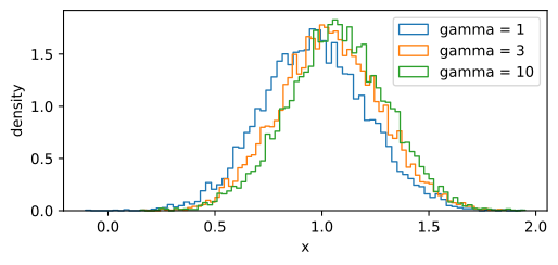
gamma =  1.0: mass right of 0: 1.000, mean 0.966, std 0.244
gamma =  3.0: mass right of 0: 1.000, mean 1.035, std 0.236
gamma = 10.0: mass right of 0: 1.000, mean 1.072, std 0.234
exact conditional: mean 0.970, std 0.243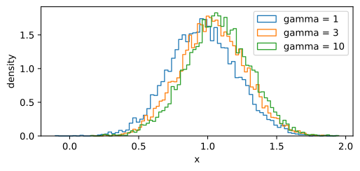
gamma =  1.0: mass right of 0: 1.000, mean 0.966, std 0.244
gamma =  3.0: mass right of 0: 1.000, mean 1.035, std 0.236
gamma = 10.0: mass right of 0: 1.000, mean 1.072, std 0.234
exact conditional: mean 0.970, std 0.243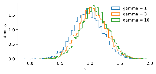
gamma =  1.0: mass right of 0: 1.000, mean 0.966, std 0.244
gamma =  3.0: mass right of 0: 1.000, mean 1.035, std 0.236
gamma = 10.0: mass right of 0: 1.000, mean 1.072, std 0.234
exact conditional: mean 0.970, std 0.243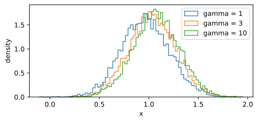
The printout measures the tilt. At \(\gamma = 1\) the finite-step sampler closely approximates the exact conditional: mean \(0.966\) against the analytic \(0.970\), standard deviation \(0.244\) against \(0.243\), and all of the mass in the right mode, where the unconditional mixture would put only half of it. Pushing \(\gamma\) to \(3\) and \(10\) has no more mass to reallocate, so it distorts the surviving mode instead: the mean slides from \(0.97\) to \(1.04\) to \(1.07\), away from the class boundary (“more prototypically \(y\)”) while the histogram narrows slightly. This shift and narrowing illustrate the preceding caveat: for \(\gamma > 1\) the samples track no noised marginal of any clean distribution; the tilt is its own object, more emphatic and less diverse than the class it names.
29.4.3 Flow Matching and Rectified Flow
29.4.3.1 Probability Paths and Velocity Fields
Diffusion derives a bridge between noise and data from a stochastic process and then reverses it. Flow matching (Lipman et al. 2023) instead prescribes a family of densities \((p_t)_{t \in [0, 1]}\) with \(p_0\) = noise and \(p_1\) = data (a probability path) and learn the velocity field that transports mass along it. Recall from Section 29.3.3 that a velocity field \(\mathbf{u}_t\) realizes the path iff the pair satisfies the continuity equation \(\partial_t p_t = -\nabla \cdot (p_t\, \mathbf{u}_t)\). If we can fit \(\mathbf{v}_{\boldsymbol{\theta}} \approx \mathbf{u}_t\), generation is a plain ODE solve of \(\dot{\mathbf{x}} = \mathbf{v}_{\boldsymbol{\theta}}(\mathbf{x}, t)\) from \(\mathbf{x}_0 \sim p_0\): a continuous normalizing flow (Section 29.1.5) trained without ever simulating the ODE. The natural objective is the flow-matching loss
\[ \mathcal{L}_{\mathrm{FM}}(\boldsymbol{\theta}) = \mathbb{E}_{t \sim \mathcal{U}[0,1],\ \mathbf{x} \sim p_t} \left[\, \left\| \mathbf{v}_{\boldsymbol{\theta}}(\mathbf{x}, t) - \mathbf{u}_t(\mathbf{x}) \right\|^2 \right], \tag{29.4.13}\]
Like explicit score matching, this objective contains an unknown marginal field, the velocity \(\mathbf{u}_t\). A tractable alternative constructs the path out of conditional paths, one per data point: pick \(p_t(\mathbf{x} \mid \mathbf{z})\), a little moving blob that starts spread as noise and collapses onto the conditioning variable \(\mathbf{z}\) (say, a data point \(\mathbf{x}_1\), or a pair \((\mathbf{x}_0, \mathbf{x}_1)\)), whose conditional velocity \(\mathbf{u}_t(\mathbf{x} \mid \mathbf{z})\) we can write down, and let the marginal path be the mixture \(p_t(\mathbf{x}) = \int p_t(\mathbf{x} \mid \mathbf{z})\, q(\mathbf{z})\, d\mathbf{z}\).
Proposition (the marginal velocity is a posterior mean). Suppose each conditional pair satisfies the continuity equation, \(\partial_t p_t(\mathbf{x} \mid \mathbf{z}) = -\nabla \cdot \left( p_t(\mathbf{x} \mid \mathbf{z})\, \mathbf{u}_t(\mathbf{x} \mid \mathbf{z}) \right)\), with integrability sufficient to differentiate the mixture under the integral sign, and define on \(\{p_t > 0\}\) the marginal velocity
\[ \mathbf{u}_t(\mathbf{x}) = \mathbb{E}\left[ \mathbf{u}_t(\mathbf{x} \mid \mathbf{z}) \mid \mathbf{x}_t = \mathbf{x} \right] = \int \mathbf{u}_t(\mathbf{x} \mid \mathbf{z})\, \frac{p_t(\mathbf{x} \mid \mathbf{z})\, q(\mathbf{z})}{p_t(\mathbf{x})}\, d\mathbf{z}. \tag{29.4.14}\]
Then \((p_t, \mathbf{u}_t)\) satisfies the continuity equation: the averaged field transports the averaged path.
Proof. Differentiate the mixture under the integral sign and substitute the conditional continuity equation:
\[ \partial_t p_t(\mathbf{x}) = \int \partial_t p_t(\mathbf{x} \mid \mathbf{z})\, q(\mathbf{z})\, d\mathbf{z} = -\nabla \cdot \int p_t(\mathbf{x} \mid \mathbf{z})\, \mathbf{u}_t(\mathbf{x} \mid \mathbf{z})\, q(\mathbf{z})\, d\mathbf{z} = -\nabla \cdot \left( p_t(\mathbf{x})\, \mathbf{u}_t(\mathbf{x}) \right), \]
where the last step is the definition Equation 29.4.14. \(\blacksquare\)
29.4.3.2 The Conditional Flow Matching Theorem
The target is an intractable posterior mean Equation 29.4.14 of a tractable per-sample quantity, so the regression lemma Equation 29.4.5 applies. Define the conditional flow matching loss, which needs only samples \((t, \mathbf{z}, \mathbf{x})\) and the closed-form conditional velocity:
\[ \mathcal{L}_{\mathrm{CFM}}(\boldsymbol{\theta}) = \mathbb{E}_{t,\ \mathbf{z} \sim q,\ \mathbf{x} \sim p_t(\cdot \mid \mathbf{z})} \left[\, \left\| \mathbf{v}_{\boldsymbol{\theta}}(\mathbf{x}, t) - \mathbf{u}_t(\mathbf{x} \mid \mathbf{z}) \right\|^2 \right]. \tag{29.4.15}\]
Theorem (CFM trains the marginal field). Under the integrability needed for Equation 29.4.14 to exist,
\[ \mathcal{L}_{\mathrm{CFM}}(\boldsymbol{\theta}) = \mathcal{L}_{\mathrm{FM}}(\boldsymbol{\theta}) + C \]
with \(C\) independent of \(\boldsymbol{\theta}\). In particular \(\nabla_{\boldsymbol{\theta}} \mathcal{L}_{\mathrm{CFM}} = \nabla_{\boldsymbol{\theta}} \mathcal{L}_{\mathrm{FM}}\): the two objectives have identical gradients and identical minimizers (Lipman et al. 2023; Tong et al. 2024).
Proof. Apply the regression lemma Equation 29.4.5 with \(X = (\mathbf{x}, t)\) where \(\mathbf{x} \sim p_t(\cdot \mid \mathbf{z})\), and \(Y = \mathbf{u}_t(\mathbf{x} \mid \mathbf{z})\). The marginal distribution of \(X\) is \(t \sim \mathcal{U}[0,1]\), \(\mathbf{x} \sim p_t\), and the conditional mean of \(Y\) given \(X = (\mathbf{x}, t)\) is, by definition, Equation 29.4.14, the marginal velocity. The lemma splits \(\mathcal{L}_{\mathrm{CFM}}\) into \(\mathbb{E}\| \mathbf{v}_{\boldsymbol{\theta}}(X) - \mathbf{u}_t(\mathbf{x}) \|^2 = \mathcal{L}_{\mathrm{FM}}\) plus the posterior variance term \(C = \mathbb{E}\| Y - \mathbf{u}_t(\mathbf{x}) \|^2\), which does not involve \(\boldsymbol{\theta}\). \(\blacksquare\)
This proof has the same structure as Vincent’s theorem, with (score of the noising kernel \(\to\) marginal score) replaced by (conditional velocity \(\to\) marginal velocity). Denoising score matching is conditional flow matching for the score field. The flow-matching formulation extends this argument to general velocity fields. As before, the theorem’s constant \(C\) is the conditional variance of the regression target. The population CFM loss therefore need not vanish even for a perfect marginal field; its value depends on the chosen path, coupling, and target parameterization.
29.4.3.3 Relations Among Score, Noise, and Velocity
Diffusion trains a score, whereas flow matching trains a velocity. For the Gaussian paths used in practice, these quantities determine one another through explicit transformations. Condition on a data point and take the Gaussian path
\[ \mathbf{x}_t = \alpha_t\, \mathbf{x}_1 + \sigma_t\, \boldsymbol{\epsilon}, \qquad \boldsymbol{\epsilon} \sim \mathcal{N}(\mathbf{0}, I), \]
with smooth schedules \((\alpha_t, \sigma_t)\): on the flow-matching clock \((\alpha_0, \sigma_0) = (0, 1)\) and \((\alpha_1, \sigma_1) = (1, 0)\); on the diffusion clock, write \(\mathbf{x}_0\) for the data point and swap the boundary conditions, and every formula below holds verbatim.
Proposition (score–velocity identity). For the Gaussian path above, at any \(t\) with \(\alpha_t, \sigma_t > 0\) and on \(\{p_t > 0\}\), the marginal velocity Equation 29.4.14 and the marginal score determine each other:
\[ \mathbf{u}_t(\mathbf{x}) = \frac{\dot{\alpha}_t}{\alpha_t}\, \mathbf{x} - \left( \sigma_t \dot{\sigma}_t - \sigma_t^2\, \frac{\dot{\alpha}_t}{\alpha_t} \right) \nabla \log p_t(\mathbf{x}). \tag{29.4.16}\]
Proof. Both sides are posterior expectations given \(\mathbf{x}_t = \mathbf{x}\), and both are affine in the same one: write \(\hat{\mathbf{x}}_1 = \mathbb{E}[\mathbf{x}_1 \mid \mathbf{x}_t = \mathbf{x}]\). Differentiating the path gives the conditional velocity \(\dot{\mathbf{x}}_t = \dot{\alpha}_t \mathbf{x}_1 + \dot{\sigma}_t \boldsymbol{\epsilon}\) with \(\boldsymbol{\epsilon} = (\mathbf{x} - \alpha_t \mathbf{x}_1)/\sigma_t\), so taking the posterior mean in Equation 29.4.14,
\[ \mathbf{u}_t(\mathbf{x}) = \frac{\dot{\sigma}_t}{\sigma_t}\, \mathbf{x} + \left( \dot{\alpha}_t - \alpha_t\, \frac{\dot{\sigma}_t}{\sigma_t} \right) \hat{\mathbf{x}}_1. \]
Meanwhile the marginal score is the posterior mean of the conditional scores (Vincent’s theorem, verbatim), and the conditional score of the kernel \(\mathcal{N}(\alpha_t \mathbf{x}_1, \sigma_t^2 I)\) is \((\alpha_t \mathbf{x}_1 - \mathbf{x})/\sigma_t^2\), so Tweedie’s formula for this kernel reads
\[ \nabla \log p_t(\mathbf{x}) = \mathbb{E}\left[ \frac{\alpha_t \mathbf{x}_1 - \mathbf{x}}{\sigma_t^2} \,\middle|\, \mathbf{x}_t = \mathbf{x} \right] = \frac{\alpha_t \hat{\mathbf{x}}_1 - \mathbf{x}}{\sigma_t^2}, \qquad \textrm{i.e.}\quad \hat{\mathbf{x}}_1 = \frac{\mathbf{x} + \sigma_t^2\, \nabla \log p_t(\mathbf{x})}{\alpha_t}. \]
Substitute this into the velocity display above and collect the \(\mathbf{x}\) and \(\nabla \log p_t\) terms to obtain Equation 29.4.16. \(\blacksquare\)
The same posterior mean \(\hat{\mathbf{x}}_1\) underlies the common parameterizations, so they are inter-convertible by \(t\)-dependent affine maps of the same posterior mean:
| Network predicts | Posterior meaning | From the score \(\mathbf{s} = \nabla \log p_t\) |
|---|---|---|
| score \(\mathbf{s}_{\boldsymbol{\theta}}\) | \(\nabla \log p_t(\mathbf{x})\) | \(\mathbf{s}\) |
| noise \(\hat{\boldsymbol{\epsilon}}\) | \(\mathbb{E}[\boldsymbol{\epsilon} \mid \mathbf{x}_t = \mathbf{x}]\) | \(-\sigma_t\, \mathbf{s}\) |
| clean point \(\hat{\mathbf{x}}_1\) | \(\mathbb{E}[\mathbf{x}_1 \mid \mathbf{x}_t = \mathbf{x}]\) | \((\mathbf{x} + \sigma_t^2\, \mathbf{s})/\alpha_t\) (Tweedie) |
| velocity \(\mathbf{v}_{\boldsymbol{\theta}}\) | \(\mathbb{E}[\dot{\mathbf{x}}_t \mid \mathbf{x}_t = \mathbf{x}]\) | the identity Equation 29.4.16 |
| \(v\)-prediction \(\hat{\mathbf{v}}\) | \(\mathbb{E}[\alpha_t \boldsymbol{\epsilon} - \sigma_t \mathbf{x}_1 \mid \mathbf{x}_t = \mathbf{x}]\) | \(-\tfrac{\sigma_t}{\alpha_t}\, \mathbf{x} - \sigma_t\, \tfrac{\alpha_t^2 + \sigma_t^2}{\alpha_t}\, \mathbf{s}\) |
Target choice changes the conditioning of the regression problem. Near the data end, the sampled conditional-score target \(-\boldsymbol{\epsilon}/\sigma_t\) has scale \(1/\sigma_t\); the marginal score need not. Indeed the optimal noise prediction is \(\mathbb{E}[\boldsymbol{\epsilon}\mid\mathbf{x}_t] =-\sigma_t\nabla\log p_t(\mathbf{x}_t)\), which can shrink to zero when the clean density has a finite score. Noise prediction nevertheless keeps the sampled training target at unit scale. Near the noise end, \(\hat{\mathbf{x}}_1=(\mathbf{x}-\sigma_t\hat{\boldsymbol{\epsilon}})/\alpha_t\) amplifies noise-prediction error by \(1/\alpha_t\). Under common normalized schedules, the \(v\)-prediction target \(\alpha_t\boldsymbol{\epsilon}-\sigma_t\mathbf{x}_1\) keeps the two sampled components on comparable scales, which motivates its use in distillation (Salimans and Ho 2022). These are conditioning tendencies, not identities about every data distribution.
A useful schedule coordinate is the log signal-to-noise ratio \(\rho_t=\log(\alpha_t^2/\sigma_t^2)\), using a different symbol from the loss weight. After the corresponding state rescaling, schedules that traverse the same monotone range of \(\rho\) describe the same family of noised marginals up to time reparameterization (Kingma et al. 2021). Their velocity fields also acquire the derivative of that reparameterization, so training weights and numerical difficulty need not be the same. EDM’s \(\alpha_t\equiv1\), \(\sigma_t=t\) parameterization is a closely related variance-exploding coordinate choice designed jointly with its preconditioning and sampler (Karras et al. 2022).
The identity is checkable to machine precision with the section’s own mixture: at a fixed \(t\), compute the marginal velocity once from the posterior mean (route one, no score in sight) and once from the dictionary formula Equation 29.4.16 with the analytic score (route two, no velocity in sight).
t = 0.6                                       # one fixed time, cosine schedule
alpha, sigma = np.sin(np.pi * t / 2), np.cos(np.pi * t / 2)
dalpha, dsigma = np.pi / 2 * sigma, -np.pi / 2 * alpha
grid = np.linspace(-4.0, 4.0, 201)
means, var0 = np.array([-2.0, 2.0]), 0.25     # the mixture of the DSM demo
vart = alpha**2 * var0 + sigma**2             # noised component variance
w = np.stack([np.exp(-(grid - alpha * m)**2 / (2 * vart)) for m in means])
w /= w.sum(0)                                 # posterior mode responsibilities
x1_hat = (w * np.stack([m + alpha * var0 / vart * (grid - alpha * m)
                        for m in means])).sum(0)          # E[x_1 | x_t]
u_posterior = dalpha * x1_hat + dsigma / sigma * (grid - alpha * x1_hat)
score = (w * np.stack([(alpha * m - grid) / vart for m in means])).sum(0)
u_dictionary = (dalpha / alpha) * grid \
    - (sigma * dsigma - sigma**2 * dalpha / alpha) * score
print(f'max |u_posterior - u_dictionary| on [-4, 4]: '
      f'{np.abs(u_posterior - u_dictionary).max():.1e}')
max |u_posterior - u_dictionary| on [-4, 4]: 3.1e-15The two routes agree to about \(10^{-15}\) (machine precision) across both modes and the low-density valley. No model was fitted: the posterior calculation does not use a score, while the alternative calculation uses the score–velocity relation. They agree because both are affine in the same posterior mean \(\hat{x}_1\). Thus noise-prediction and velocity-field implementations can represent equivalent targets.
29.4.3.4 Rectified Flow and Straight Paths
Consider a conditional path defined by a pair \(\mathbf{z} = (\mathbf{x}_0, \mathbf{x}_1)\), a noise sample and a data sample drawn independently, and connect them by a straight line traversed at constant speed:
\[ \mathbf{x}_t = (1 - t)\, \mathbf{x}_0 + t\, \mathbf{x}_1, \qquad \mathbf{u}_t(\mathbf{x}_t \mid \mathbf{z}) = \dot{\mathbf{x}}_t = \mathbf{x}_1 - \mathbf{x}_0. \tag{29.4.17}\]
The conditional velocity does not even depend on \(t\): the CFM loss Equation 29.4.15 becomes the rectified flow (equivalently, linear-path CFM) objective (Liu et al. 2023; Lipman et al. 2023)
\[ \mathcal{L}_{\mathrm{RF}}(\boldsymbol{\theta}) = \mathbb{E}_{t,\ \mathbf{x}_0 \sim p_0,\ \mathbf{x}_1 \sim p_1} \left[\, \left\| \mathbf{v}_{\boldsymbol{\theta}}\big( (1 - t) \mathbf{x}_0 + t \mathbf{x}_1,\ t \big) - (\mathbf{x}_1 - \mathbf{x}_0) \right\|^2 \right] \tag{29.4.18}\]
Training draws noise and data, interpolates between them, and regresses on the difference. (For the measure-theoretic comfort of strictly positive conditional densities, smooth the line with an infinitesimal Gaussian, \(p_t(\cdot \mid \mathbf{z}) = \mathcal{N}((1-t)\mathbf{x}_0 + t \mathbf{x}_1, \sigma_{\min}^2 I)\), and let \(\sigma_{\min} \to 0\); the limiting objective is unchanged. Gaussian conditional paths with general \((\mu_t, \sigma_t)\) schedules recover diffusion-style targets: that is how flow matching subsumes the VP path, modulo the time-reversal callout above.)
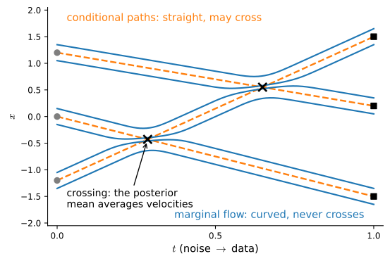
A subtlety (Figure 29.4.5): the conditional paths are straight, but the marginal flow that the network learns is generally curved. Two straight segments that cross at \((\mathbf{x}, t)\) feed the posterior mean Equation 29.4.14 two different directions, and the learned field (which, like any function, can have only one value there) averages them. An ODE’s trajectories cannot meet at the same \((\mathbf{x}, t)\) (uniqueness, Section 29.1.1.3), so the learned flow bends to avoid the collisions that the conditional segments ignore. The independent coupling of \(\mathbf{x}_0\) and \(\mathbf{x}_1\) can produce many crossings and a curved marginal field, which can increase low-order solver error. Reflow (Liu et al. 2023) attacks the coupling: after training, generate pairs \((\mathbf{x}_0, \hat{\mathbf{x}}_1)\) by running the current model’s ODE, and retrain on this new coupling, in which start and end points are already dynamically matched. For the exact population rectification operator, the theorem preserves endpoint marginals and does not increase convex transport costs. A finite network trained on numerically generated endpoints only approximates this operator. In the straight limit, one Euler step is exact (the local truncation error of Euler is controlled by the curvature \(\ddot{\mathbf{x}}\) along trajectories, Section 29.1.3); this is the mathematics behind few-step and one-step generators distilled from flows.
29.4.3.5 Gaussian to Two Moons, Four Ways
The numerical example uses a two-moons target (two interleaved crescents, a classic stress test for mode-splitting) generated in a few lines of NumPy; the source is a standard 2-D Gaussian. We also define the energy distance (Székely and Rizzo 2013)
\[ \mathcal{E}(P, Q) = \left( 2\, \mathbb{E}\|X - Y\| - \mathbb{E}\|X - X'\| - \mathbb{E}\|Y - Y'\| \right)^{1/2}, \]
an MMD-style two-sample discrepancy (Section 28.2.3.2) that is zero iff the distributions agree; we use its square, on \(2048\)-point samples, to compare generated samples with a held-out target sample throughout.
def two_moons(n, rng, noise=0.07):
    t = rng.uniform(0.0, np.pi, n)
    m = rng.integers(0, 2, n)                      # which moon
    X = np.stack([np.cos(t) * (1 - 2 * m) + m,
                  np.sin(t) * (1 - 2 * m) + 0.5 * m], axis=1)
    return X + noise * rng.standard_normal((n, 2))

rng = np.random.default_rng(0)
raw = two_moons(8192, rng)
mu, sd = raw.mean(0), raw.std(0)
moons = (raw - mu) / sd                            # standardized training data
held_out = (two_moons(2048, np.random.default_rng(1)) - mu) / sd

def energy_distance(a, b):                         # squared energy distance
    d = lambda u, v: np.linalg.norm(u[:, None, :] - v[None, :, :], axis=-1).mean()
    return 2 * d(a, b) - d(a, a) - d(b, b)

print(f'training set {moons.shape}; energy distance of a fresh sample '
      f'to the held-out set: {energy_distance(moons[:2048], held_out):.4f}')
training set (8192, 2); energy distance of a fresh sample to the held-out set: 0.0014The fresh-sample-to-held-out value (\(\approx 0.001\) in this draw) is a finite-sample reference for the metric, not a universal lower bound. The model is a velocity field \(\mathbf{v}_{\boldsymbol{\theta}} : \mathbb{R}^2 \times [0, 1] \to \mathbb{R}^2\) as a \(3 \to 64 \to 64 \to 2\) tanh MLP, trained for \(4000\) Adam steps on the rectified-flow objective Equation 29.4.18. Each batch follows the same construction: sample \(\mathbf{x}_0\), \(\mathbf{x}_1\), and \(t\); interpolate; regress on \(\mathbf{x}_1 - \mathbf{x}_0\). This is the section’s second training loop (the NumPy score network was the first), and it takes a few seconds on a CPU.
torch.manual_seed(0)
data = torch.tensor(moons, dtype=torch.float32)
net = nn.Sequential(nn.Linear(3, 64), nn.Tanh(), nn.Linear(64, 64), nn.Tanh(),
                    nn.Linear(64, 2))
opt = torch.optim.Adam(net.parameters(), lr=3e-3)
for step in range(4001):
    x1 = data[torch.randint(0, len(data), (256,))]
    x0, t = torch.randn(256, 2), torch.rand(256, 1)
    xt = (1 - t) * x0 + t * x1
    loss = ((net(torch.cat([xt, t], 1)) - (x1 - x0))**2).mean()
    opt.zero_grad()
    loss.backward()
    opt.step()
    if step % 1000 == 0:
        print(f'step {step:4d}: CFM loss {loss.item():.3f}')
step 0: CFM loss 2.157
step 1000: CFM loss 1.351
step 2000: CFM loss 1.526
step 3000: CFM loss 1.321
step 4000: CFM loss 1.323tf.keras.utils.set_random_seed(0)
data = tf.constant(moons, tf.float32)
net = tf.keras.Sequential([tf.keras.layers.Dense(64, 'tanh'),
tf.keras.layers.Dense(64, 'tanh'),
tf.keras.layers.Dense(2)])
opt = tf.keras.optimizers.Adam(3e-3)
@tf.function
def train_step():
x1 = tf.gather(data, tf.random.uniform((256,), 0, len(data), tf.int32))
x0 = tf.random.normal((256, 2))
t = tf.random.uniform((256, 1))
xt = (1 - t) * x0 + t * x1
with tf.GradientTape() as tape:
v = net(tf.concat([xt, t], 1))
loss = tf.reduce_mean((v - (x1 - x0))**2)
grads = tape.gradient(loss, net.trainable_variables)
opt.apply_gradients(zip(grads, net.trainable_variables))
return loss
for step in range(4001):
loss = train_step()
if step % 1000 == 0:
print(f'step {step:4d}: CFM loss {float(loss):.3f}')step 0: CFM loss 2.011
step 1000: CFM loss 1.556
step 2000: CFM loss 1.561
step 3000: CFM loss 1.162
step 4000: CFM loss 1.552def init_mlp(key, sizes=(3, 64, 64, 2)):
keys = jax.random.split(key, len(sizes) - 1)
return [(jax.random.normal(k, (i, o)) / jnp.sqrt(i), jnp.zeros(o))
for k, i, o in zip(keys, sizes[:-1], sizes[1:])]
def mlp(params, x):
for W, b in params[:-1]:
x = jnp.tanh(x @ W + b)
return x @ params[-1][0] + params[-1][1]
data = jnp.asarray(moons, dtype=jnp.float32)
def cfm_loss(params, key):
k1, k2, k3 = jax.random.split(key, 3)
x1 = data[jax.random.randint(k1, (256,), 0, len(data))]
x0 = jax.random.normal(k2, (256, 2))
t = jax.random.uniform(k3, (256, 1))
xt = (1 - t) * x0 + t * x1
v = mlp(params, jnp.concatenate([xt, t], axis=1))
return ((v - (x1 - x0))**2).mean()
opt = optax.adam(3e-3)
params = init_mlp(jax.random.key(0))
state = opt.init(params)
@jax.jit
def train(params, state, key):
def step(carry, k):
params, state = carry
loss, grads = jax.value_and_grad(cfm_loss)(params, k)
updates, state = opt.update(grads, state)
return (optax.apply_updates(params, updates), state), loss
return jax.lax.scan(step, (params, state), jax.random.split(key, 4000))
(params, state), losses = train(params, state, jax.random.key(1))
print(f'CFM loss: step 0 {losses[0]:.3f} -> step 4000 {losses[-1]:.3f}')CFM loss: step 0 1.908 -> step 4000 1.402mxnp.random.seed(0)
data = mxnp.array(moons)
net = gluon.nn.Sequential()
net.add(gluon.nn.Dense(64, activation='tanh'),
gluon.nn.Dense(64, activation='tanh'),
gluon.nn.Dense(2))
net.initialize(init.Xavier())
trainer = gluon.Trainer(net.collect_params(), 'adam', {'learning_rate': 3e-3})
for step in range(4001):
x1 = data[mxnp.random.randint(0, len(data), (256,))]
x0 = mxnp.random.normal(0, 1, (256, 2))
t = mxnp.random.uniform(0, 1, (256, 1))
xt = (1 - t) * x0 + t * x1
with autograd.record():
v = net(mxnp.concatenate([xt, t], axis=1))
loss = ((v - (x1 - x0))**2).mean()
loss.backward()
trainer.step(1)
if step % 1000 == 0:
print(f'step {step:4d}: CFM loss {float(loss):.3f}')step 0: CFM loss 2.125[22:56:57] /home/smola/mxnet/src/base.cc:48: GPU context requested, but no GPUs found.step 1000: CFM loss 1.590
step 2000: CFM loss 1.459
step 3000: CFM loss 1.419
step 4000: CFM loss 1.427The loss falls from about \(2\) to about \(1.3\) and then plateaus, as the CFM theorem predicts. This value reflects the conditional variance of \(\mathbf{x}_1 - \mathbf{x}_0\) around its posterior mean rather than zero. Sampling is an Euler loop (Section 29.1.3) integrating \(\dot{\mathbf{x}} = \mathbf{v}_{\boldsymbol{\theta}}(\mathbf{x}, t)\) from \(t = 0\) to \(1\). For this trained field, the panels show how the selected metric and sample geometry change with step count: one step produces a smeared blob, two steps a bent ellipse, eight steps recognizable moons, thirty-two steps sharp ones.
def euler_sample(n, steps, seed=2):
    g = torch.Generator().manual_seed(seed)
    q = torch.randn(n, 2, generator=g)
    for k in range(steps):
        t = torch.full((n, 1), k / steps)
        with torch.no_grad():
            q = q + (1.0 / steps) * net(torch.cat([q, t], 1))
    return q.numpy()
def euler_sample(n, steps, seed=2):
q = tf.random.stateless_normal((n, 2), [seed, 0])
for k in range(steps):
t = tf.fill((n, 1), tf.cast(k / steps, tf.float32))
q = q + (1.0 / steps) * net(tf.concat([q, t], 1))
return q.numpy()velocity = jax.jit(
lambda params, q, t: mlp(params, jnp.concatenate([q, t], axis=1)))
def euler_sample(n, steps, seed=2):
q = jax.random.normal(jax.random.key(seed), (n, 2))
for k in range(steps):
q = q + (1.0 / steps) * velocity(params, q, jnp.full((n, 1), k / steps))
return np.asarray(q)def euler_sample(n, steps, seed=2):
mxnp.random.seed(seed)
q = mxnp.random.normal(0, 1, (n, 2))
for k in range(steps):
t = mxnp.full((n, 1), k / steps)
q = q + (1.0 / steps) * net(mxnp.concatenate([q, t], axis=1))
return q.asnumpy()panels = [('data', moons[:2048])] + [
(f'{K} step(s)', euler_sample(2048, K)) for K in (1, 2, 8, 32)]
fig, axes = d2l.plt.subplots(1, 5, figsize=(11, 2.4), sharex=True, sharey=True)
for ax, (title, s) in zip(axes, panels):
ax.scatter(s[:, 0], s[:, 1], s=1)
ax.set_title(title)
ax.set_xlim(-2.5, 2.5), ax.set_ylim(-2.5, 2.5)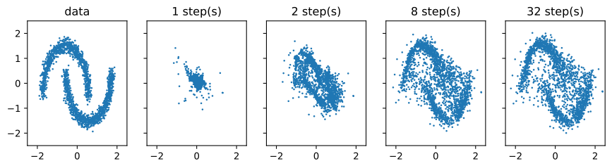
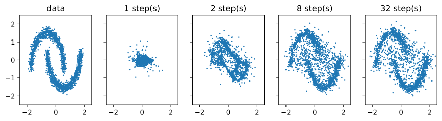
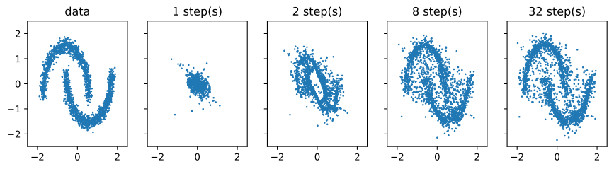
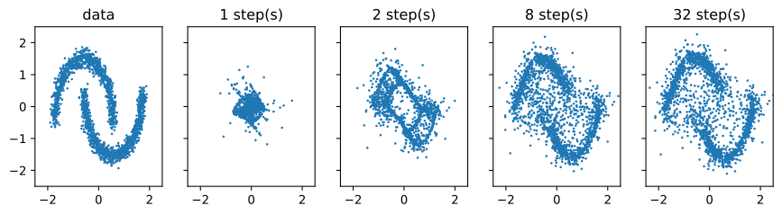
For this model, a few Euler steps already recover the main geometry, while the remaining discrepancy decreases more slowly. The next section gives a precise energy interpretation of straight paths; it does not equate that energy with a universal step count.
29.4.3.6 The Effect of One Reflow Round
Before leaving the trained model, we can test the intended effect of reflow on the learned paths. Apply the procedure of Section 29.4.3.4: draw fresh noise \(\mathbf{z}\), integrate the trained ODE for \(32\) Euler steps to obtain the model’s own endpoint \(\hat{\mathbf{x}}_1(\mathbf{z})\), and retrain the same architecture on the coupled pairs \((\mathbf{z}, \hat{\mathbf{x}}_1(\mathbf{z}))\) in place of independent ones. If the new couplings rarely cross, the retrained flow should be nearly straight, and a nearly straight flow should sample well in one Euler step.
g = torch.Generator().manual_seed(3)
z = torch.randn(8192, 2, generator=g)              # noise endpoints, kept
x1_hat = z.clone()
for k in range(32):                                # the model's own couplings
    t = torch.full((8192, 1), k / 32)
    with torch.no_grad():
        x1_hat = x1_hat + (1.0 / 32) * net(torch.cat([x1_hat, t], 1))
net2 = nn.Sequential(nn.Linear(3, 64), nn.Tanh(), nn.Linear(64, 64), nn.Tanh(),
                     nn.Linear(64, 2))
opt2 = torch.optim.Adam(net2.parameters(), lr=3e-3)
for step in range(4001):
    i = torch.randint(0, len(z), (256,))
    x0, x1 = z[i], x1_hat[i]                       # the same pair, never re-paired
    t = torch.rand(256, 1)
    xt = (1 - t) * x0 + t * x1
    loss = ((net2(torch.cat([xt, t], 1)) - (x1 - x0))**2).mean()
    opt2.zero_grad()
    loss.backward()
    opt2.step()
print(f'final reflow loss {loss.item():.3f}')

def euler_sample2(n, steps, seed=2):
    g = torch.Generator().manual_seed(seed)
    q = torch.randn(n, 2, generator=g)
    for k in range(steps):
        t = torch.full((n, 1), k / steps)
        with torch.no_grad():
            q = q + (1.0 / steps) * net2(torch.cat([q, t], 1))
    return q.numpy()

for K in (1, 2, 32):
    print(f'{K:2d} step(s): energy distance  '
          f'CFM {energy_distance(euler_sample(2048, K), held_out):.3f}  ->  '
          f'reflow {energy_distance(euler_sample2(2048, K), held_out):.3f}')
final reflow loss 0.001
1 step(s): energy distance CFM 0.676 -> reflow 0.016
2 step(s): energy distance CFM 0.163 -> reflow 0.015
32 step(s): energy distance CFM 0.014 -> reflow 0.016tf.keras.utils.set_random_seed(3)
z = tf.random.stateless_normal((8192, 2), [3, 0]) # noise endpoints, kept
x1_hat = z
for k in range(32): # the model's own couplings
t = tf.fill((8192, 1), tf.cast(k / 32, tf.float32))
x1_hat = x1_hat + (1.0 / 32) * net(tf.concat([x1_hat, t], 1))
net2 = tf.keras.Sequential([tf.keras.layers.Dense(64, 'tanh'),
tf.keras.layers.Dense(64, 'tanh'),
tf.keras.layers.Dense(2)])
opt2 = tf.keras.optimizers.Adam(3e-3)
@tf.function
def reflow_step():
i = tf.random.uniform((256,), 0, len(z), tf.int32)
x0, x1 = tf.gather(z, i), tf.gather(x1_hat, i) # the same pair, never re-paired
t = tf.random.uniform((256, 1))
xt = (1 - t) * x0 + t * x1
with tf.GradientTape() as tape:
v = net2(tf.concat([xt, t], 1))
loss = tf.reduce_mean((v - (x1 - x0))**2)
grads = tape.gradient(loss, net2.trainable_variables)
opt2.apply_gradients(zip(grads, net2.trainable_variables))
return loss
for step in range(4001):
loss = reflow_step()
print(f'final reflow loss {float(loss):.3f}')
def euler_sample2(n, steps, seed=2):
q = tf.random.stateless_normal((n, 2), [seed, 0])
for k in range(steps):
t = tf.fill((n, 1), tf.cast(k / steps, tf.float32))
q = q + (1.0 / steps) * net2(tf.concat([q, t], 1))
return q.numpy()
for K in (1, 2, 32):
print(f'{K:2d} step(s): energy distance '
f'CFM {energy_distance(euler_sample(2048, K), held_out):.3f} -> '
f'reflow {energy_distance(euler_sample2(2048, K), held_out):.3f}')final reflow loss 0.003
1 step(s): energy distance CFM 0.582 -> reflow 0.006
2 step(s): energy distance CFM 0.138 -> reflow 0.005
32 step(s): energy distance CFM 0.007 -> reflow 0.005z = jax.random.normal(jax.random.key(3), (8192, 2)) # noise endpoints, kept
x1_hat = z
for k in range(32): # the model's own couplings
x1_hat = x1_hat + (1.0 / 32) * velocity(params, x1_hat,
jnp.full((8192, 1), k / 32))
def reflow_loss(params2, key):
k1, k2 = jax.random.split(key)
i = jax.random.randint(k1, (256,), 0, len(z))
x0, x1 = z[i], x1_hat[i] # the same pair, never re-paired
t = jax.random.uniform(k2, (256, 1))
xt = (1 - t) * x0 + t * x1
v = mlp(params2, jnp.concatenate([xt, t], axis=1))
return ((v - (x1 - x0))**2).mean()
params2 = init_mlp(jax.random.key(4))
state2 = opt.init(params2)
@jax.jit
def retrain(params2, state2, key):
def step(carry, k):
params2, state2 = carry
loss, grads = jax.value_and_grad(reflow_loss)(params2, k)
updates, state2 = opt.update(grads, state2)
return (optax.apply_updates(params2, updates), state2), loss
return jax.lax.scan(step, (params2, state2), jax.random.split(key, 4000))
(params2, state2), losses = retrain(params2, state2, jax.random.key(5))
print(f'final reflow loss {losses[-1]:.3f}')
def euler_sample2(n, steps, seed=2):
q = jax.random.normal(jax.random.key(seed), (n, 2))
for k in range(steps):
q = q + (1.0 / steps) * velocity(params2, q, jnp.full((n, 1), k / steps))
return np.asarray(q)
for K in (1, 2, 32):
print(f'{K:2d} step(s): energy distance '
f'CFM {energy_distance(euler_sample(2048, K), held_out):.3f} -> '
f'reflow {energy_distance(euler_sample2(2048, K), held_out):.3f}')final reflow loss 0.001
1 step(s): energy distance CFM 0.657 -> reflow 0.005
2 step(s): energy distance CFM 0.175 -> reflow 0.004
32 step(s): energy distance CFM 0.004 -> reflow 0.004mxnp.random.seed(3)
z = mxnp.random.normal(0, 1, (8192, 2)) # noise endpoints, kept
x1_hat = z.copy()
for k in range(32): # the model's own couplings
t = mxnp.full((8192, 1), k / 32)
x1_hat = x1_hat + (1.0 / 32) * net(mxnp.concatenate([x1_hat, t], axis=1))
net2 = gluon.nn.Sequential()
net2.add(gluon.nn.Dense(64, activation='tanh'),
gluon.nn.Dense(64, activation='tanh'),
gluon.nn.Dense(2))
net2.initialize(init.Xavier())
trainer2 = gluon.Trainer(net2.collect_params(), 'adam', {'learning_rate': 3e-3})
for step in range(4001):
i = mxnp.random.randint(0, len(z), (256,))
x0, x1 = z[i], x1_hat[i] # the same pair, never re-paired
t = mxnp.random.uniform(0, 1, (256, 1))
xt = (1 - t) * x0 + t * x1
with autograd.record():
v = net2(mxnp.concatenate([xt, t], axis=1))
loss = ((v - (x1 - x0))**2).mean()
loss.backward()
trainer2.step(1)
print(f'final reflow loss {float(loss):.3f}')
def euler_sample2(n, steps, seed=2):
mxnp.random.seed(seed)
q = mxnp.random.normal(0, 1, (n, 2))
for k in range(steps):
t = mxnp.full((n, 1), k / steps)
q = q + (1.0 / steps) * net2(mxnp.concatenate([q, t], axis=1))
return q.asnumpy()
for K in (1, 2, 32):
print(f'{K:2d} step(s): energy distance '
f'CFM {energy_distance(euler_sample(2048, K), held_out):.3f} -> '
f'reflow {energy_distance(euler_sample2(2048, K), held_out):.3f}')final reflow loss 0.003
1 step(s): energy distance CFM 0.603 -> reflow 0.003
2 step(s): energy distance CFM 0.129 -> reflow 0.003
32 step(s): energy distance CFM 0.003 -> reflow 0.003In this run, one Euler step of the reflowed model scores \(0.016\), close to the original model’s \(32\)-step value of \(0.014\) in this finite comparison, and about forty times smaller than the original one-step value \(0.676\). The training loss also falls to about \(0.001\) instead of plateauing near \(1.3\). This is consistent with lower conditional-target variance under the model-generated coupling, together with the fit achieved by the second network; the experiment does not estimate these contributions separately. Two caveats remain. The exact population rectification operator preserves endpoint marginals and does not increase convex transport costs; progressive straightening concerns repeated idealized rounds. What we measured is one finite round of an imperfectly trained model. Moreover, the retrained target is the model’s \(32\)-step endpoint law, not the data law, so the first model’s bias is inherited by the second. The experiment therefore demonstrates the mechanism on this two-dimensional problem; it does not establish one-step equivalence for other models or datasets.
29.4.4 Optimal Transport and Straightness
Optimal transport specifies the precise sense in which straight paths can be optimal. We keep this discussion self-contained: Section 28.2.3.3 develops the Kantorovich-dual \(W_1\) picture behind WGANs, but here we need the quadratic cost and its dynamic, fluid-flow formulation.
A coupling of two distributions \(p_0, p_1\) on \(\mathbb{R}^d\) is a joint distribution \(\pi\) with marginals \(p_0\) and \(p_1\), a randomized transportation plan saying how much mass travels from each source location to each destination. The 2-Wasserstein distance is the cheapest plan under quadratic cost:
\[ W_2^2(p_0, p_1) = \min_{\pi \in \Pi(p_0, p_1)}\ \mathbb{E}_{(\mathbf{x}_0, \mathbf{x}_1) \sim \pi} \left[\, \| \mathbf{x}_1 - \mathbf{x}_0 \|^2 \right]. \tag{29.4.19}\]
(Under mild conditions, e.g. \(p_0\) with a density, the optimal plan is deterministic, a map \(\mathbf{x}_1 = T(\mathbf{x}_0)\) with \(T\) the gradient of a convex function; that is Brenier’s theorem (Brenier 1991), and we will not need it beyond intuition.) What we need is the reformulation of Equation 29.4.19 as a least-action principle over flows, due to Benamou and Brenier (2000): the static matching problem equals a minimum over exactly the objects flow matching trains.
Theorem (Benamou–Brenier, dynamic formulation). Let \(p_0\) and \(p_1\) have finite second moments. Over all pairs \((p_t, \mathbf{v}_t)\), regular enough that the flow of \(\mathbf{v}_t\) exists, satisfying the continuity equation \(\partial_t p_t = -\nabla \cdot (p_t \mathbf{v}_t)\) with the prescribed endpoints \(p_0\) and \(p_1\),
\[ W_2^2(p_0, p_1) = \min_{(p_t, \mathbf{v}_t)}\ \int_0^1 \int \| \mathbf{v}_t(\mathbf{x}) \|^2\, p_t(\mathbf{x})\, d\mathbf{x}\, dt \tag{29.4.20}\]
The squared distance is the least kinetic energy of any flow carrying \(p_0\) to \(p_1\), and the minimizing flow transports each particle along a straight line at constant speed.
Proof sketch (the lower bound, via Jensen). Take any admissible \((p_t, \mathbf{v}_t)\) and let \(\mathbf{X}_t\) solve the ODE \(\dot{\mathbf{X}}_t = \mathbf{v}_t(\mathbf{X}_t)\) with \(\mathbf{X}_0 \sim p_0\). Two facts are granted here: that this ODE is solvable, and that its law is the continuity equation’s unique solution, so that \(\mathbf{X}_t \sim p_t\) for all \(t\) (Section 29.3.3; the uniqueness argument is the probability-flow twin of Section 29.3.3.3). In particular \((\mathbf{X}_0, \mathbf{X}_1)\) is a coupling of \((p_0, p_1)\). Then
\[ \begin{aligned} W_2^2(p_0, p_1) &\le \mathbb{E} \left\| \mathbf{X}_1 - \mathbf{X}_0 \right\|^2 = \mathbb{E} \left\| \int_0^1 \mathbf{v}_t(\mathbf{X}_t)\, dt \right\|^2 \\ &\le \mathbb{E} \int_0^1 \left\| \mathbf{v}_t(\mathbf{X}_t) \right\|^2 dt = \int_0^1\!\! \int \|\mathbf{v}_t\|^2\, p_t\, d\mathbf{x}\, dt, \end{aligned} \]
where the first inequality is suboptimality of this particular coupling and the second is Jensen’s inequality (Section 26.3.3) applied to the time average inside the squared norm. So every admissible flow has kinetic energy at least \(W_2^2\). For the matching upper bound, transport along the optimal plan in straight lines at constant speed, \(\mathbf{X}_t = (1 - t) \mathbf{X}_0 + t\, \mathbf{X}_1\) with \((\mathbf{X}_0, \mathbf{X}_1) \sim \pi^\star\): its kinetic energy is \(\mathbb{E} \|\mathbf{X}_1 - \mathbf{X}_0\|^2 = W_2^2\) exactly. (When \(\pi^\star\) is a map, this displacement interpolation is realized by a genuine velocity field; smoothing handles the general case.)
The equality analysis explains straightness. For a fixed pair of endpoints, Jensen’s inequality is tight iff the particle has constant velocity, hence follows their straight segment. Attaining the global \(W_2^2\) floor additionally requires an optimal endpoint coupling. Curvature raises the kinetic energy for a fixed coupling, but straight segments under an arbitrary coupling need not be optimal transport. This distinction organizes the methods in this section:
- Diffusion / probability-flow trajectories can be curved. For a fixed endpoint coupling, curvature raises kinetic energy relative to constant-speed straight motion and can increase the leading error of a low-order solver. It does not, by itself, determine a universal step count.
- Rectified flow starts from straight conditional segments (each pair in Equation 29.4.17 is a constant-speed line), while averaging velocities at locations reached by several pairs can bend the learned marginal flow. Reflow often reduces this curvature by replacing independent pairs with pairs generated by the current model. It does not by itself certify the optimal-transport coupling; in more than one dimension, noncrossing alone implies neither straightness nor optimality.
- Minibatch OT couplings reduce inefficient pairings before training: within each batch, re-pair the noise and data samples by solving a small discrete OT problem (an assignment over \(256\) points) and run CFM on the matched pairs (Tong et al. 2024; Pooladian et al. 2023). Matched pairs often cross less, which can reduce conditional-target variance and marginal-path curvature. A minibatch plan remains an approximation, not a certificate of the Benamou–Brenier minimizer.
One caveat: exact OT in high dimension is expensive and minibatch plans are biased toward their batch, so OT-CFM and reflow are should be viewed as variance- and curvature-reduction methods whose idealized limit is the dynamic OT problem, rather than as exact \(W_2\) solvers.
29.4.5 Numerical Sampling of Learned Dynamics
Training produces a score \(\mathbf{s}_{\boldsymbol{\theta}}\) or velocity \(\mathbf{v}_{\boldsymbol{\theta}}\). Generation substitutes this function into the corresponding dynamics and integrates from the reference distribution to the data distribution,
\[ \underbrace{\dot{\mathbf{x}} = \mathbf{v}_{\boldsymbol{\theta}}(\mathbf{x}, t) \quad \textrm{or} \quad \dot{\mathbf{x}} = \mathbf{f} - \tfrac{1}{2} g^2\, \mathbf{s}_{\boldsymbol{\theta}}}_{\textrm{deterministic (ODE)}} \qquad \textrm{versus} \qquad \underbrace{d\mathbf{x} = \left[ \mathbf{f} - g^2\, \mathbf{s}_{\boldsymbol{\theta}} \right] dt + g\, d\bar{\mathbf{W}}}_{\textrm{stochastic (reverse SDE)}}, \]
with \(\mathbf{f}\) and \(g\) the forward drift and diffusion of Section 29.2 and \(\bar{\mathbf{W}}\) a reverse-time Brownian motion: the stochastic branch is Anderson’s reverse SDE Equation 29.3.19, and both branches reuse, unchanged, the solvers of Section 29.1.3 and Section 29.2.3.2. The ODE route is deterministic (the same \(\mathbf{x}_T\) yields the same sample, useful for interpolation and editing) and often works with fewer steps for suitably trained, low-curvature fields. It also supports likelihood evaluation through the continuous-normalizing-flow trace integral of Section 29.1.5; this is exact only for the exact field, divergence, and numerical integration. The SDE route injects fresh noise and can improve exploration or empirical robustness, but noise does not universally contract model or discretization error, nor does it by itself guarantee sample diversity. Predictor–corrector methods combine the two styles. The remaining numerical choice is the number of steps. The following cell measures its effect by reusing the trained two-moons velocity field and evaluates Euler sampling at increasing step counts with the squared energy distance.
steps_list = [1, 2, 4, 8, 16, 32, 64]
eds = [energy_distance(euler_sample(2048, K), held_out) for K in steps_list]
print('  '.join(f'{K}: {e:.3f}' for K, e in zip(steps_list, eds)))
d2l.plot(steps_list, eds, 'Euler steps', 'squared energy distance',
xscale='log', yscale='log')1: 0.676 2: 0.163 4: 0.048 8: 0.021 16: 0.015 32: 0.014 64: 0.014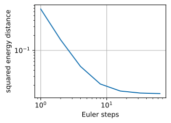
1: 0.582 2: 0.138 4: 0.027 8: 0.008 16: 0.006 32: 0.007 64: 0.007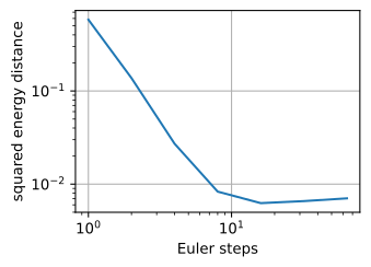
1: 0.657 2: 0.175 4: 0.044 8: 0.013 16: 0.006 32: 0.004 64: 0.003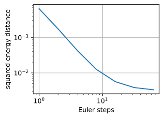
1: 0.603 2: 0.129 4: 0.024 8: 0.005 16: 0.003 32: 0.003 64: 0.003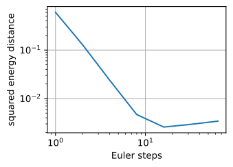
The squared energy distance falls from \(0.68\) at one step to \(0.16\) at two and \(0.05\) at four, reaches \(0.02\) by eight, and flattens near \(0.015\) from sixteen steps on (numbers from one run). The initial decline is consistent with decreasing Euler discretization error. The later plateau can combine field error with finite-sample variability of the metric; the \(0.001\) fresh-sample value printed earlier is a reference for that variability, not a universal lower bound. This experiment alone does not identify a unique error source.
Solver order is the other lever. The probability-flow ODE with the exact score of our 1-D mixture under the VP schedule lets us isolate pure discretization error, with no learning in the loop. We integrate from \(t = 1\) (noise) to \(t = 0\) (data) with Euler and with Heun’s method, the order-2 scheme of Section 29.1.3 at two field evaluations (NFE) per step, and measure the endpoint error against a finely-resolved reference solution of the same initial points.
rng = np.random.default_rng(17)
bmin, bmax = 0.1, 20.0
beta_fn = lambda t: bmin + t * (bmax - bmin)            # VP noise schedule
abar_fn = lambda t: np.exp(-(bmin * t + 0.5 * (bmax - bmin) * t**2))

def score_vp(q, t, means=(-2.0, 2.0), var=0.25):        # exact mixture score
    a = abar_fn(t)
    v = a * var + (1 - a)
    w = np.stack([np.exp(-(q - np.sqrt(a) * m)**2 / (2 * v)) for m in means])
    return (w * np.stack([(np.sqrt(a) * m - q) / v
                          for m in means])).sum(0) / w.sum(0)

def pf_ode(q, t):                                       # probability-flow ODE
    return -0.5 * beta_fn(t) * (q + score_vp(q, t))

def solve(q, K, heun=False):
    ts = np.linspace(1.0, 0.0, K + 1)
    for t1, t2 in zip(ts[:-1], ts[1:]):
        h, d1 = t2 - t1, pf_ode(q, t1)
        q = q + 0.5 * h * (d1 + pf_ode(q + h * d1, t2)) if heun \
            else q + h * d1
    return q

z = rng.standard_normal(8000)
ref = solve(z, 800, heun=True)                          # fine reference
for K in (2, 5, 10, 20, 40):
    print(f'K = {K:2d} steps: endpoint error  '
          f'Euler {np.abs(solve(z, K) - ref).mean():.4f} ({K} NFE)   '
          f'Heun {np.abs(solve(z, K, heun=True) - ref).mean():.4f} ({2 * K} NFE)')
K = 2 steps: endpoint error Euler 0.7516 (2 NFE) Heun 0.6659 (4 NFE)
K = 5 steps: endpoint error Euler 0.1215 (5 NFE) Heun 0.0808 (10 NFE)
K = 10 steps: endpoint error Euler 0.0439 (10 NFE) Heun 0.0282 (20 NFE)
K = 20 steps: endpoint error Euler 0.0203 (20 NFE) Heun 0.0085 (40 NFE)
K = 40 steps: endpoint error Euler 0.0099 (40 NFE) Heun 0.0023 (80 NFE)Doubling Euler’s steps halves its error (order one); doubling Heun’s cuts it roughly fourfold (order two), so Heun at \(20\) steps (\(40\) NFE) already beats Euler at \(40\). EDM combines this second-order correction with a schedule, preconditioning, and stochasticity choices designed as a system (Karras et al. 2022); its reported NFE improvements are empirical properties of that design, not a consequence of Heun’s order alone. Beyond that lie the topics of the main book’s generative-models chapters: consistency models, which distill a diffusion teacher into a one-step generator (Song et al. 2023); latent diffusion, which runs all of this in an autoencoder’s latent space (Rombach et al. 2022); and discrete diffusion for text (Austin et al. 2021).
29.4.5.1 Comparison of Model Families
The following table compares the probability path, regression target, and sampler used by each model family.
| Model family | Object learned | Training loss | Sampler | Stochastic? |
|---|---|---|---|---|
| DDPM (Ho et al. 2020) | \(\boldsymbol{\epsilon}_{\boldsymbol{\theta}}(\mathbf{x}_t, t)\), an equivalent score parameterization | \(\mathbb{E} \lVert \boldsymbol{\epsilon} - \boldsymbol{\epsilon}_{\boldsymbol{\theta}} \rVert^2\) (= DSM, \(\lambda(t) = 1 - \bar{\alpha}_t\)) | ancestral reverse chain; the original convention used about \(1000\) discrete levels | yes |
| Score SDE (VE/VP) (Y. Song, Sohl-Dickstein, et al. 2021) | \(\mathbf{s}_{\boldsymbol{\theta}}(\mathbf{x}, t) \approx \nabla \log p_t\) | noise-conditional DSM Equation 29.4.6 | reverse SDE via Euler–Maruyama; + Langevin corrector | yes |
| Probability-flow ODE (Y. Song, Sohl-Dickstein, et al. 2021) | same \(\mathbf{s}_{\boldsymbol{\theta}}\) (shared training) | same | ODE solver (Euler/Heun/RK); likelihood identity for exact score, terminal density, divergence, and integration | no |
| DDIM (J. Song et al. 2021) | same \(\boldsymbol{\epsilon}_{\boldsymbol{\theta}}\) as DDPM (no retraining) | same as DDPM | deterministic update Equation 29.4.10 on a sparse time grid | no (\(\eta\) interpolates) |
| Flow matching / rectified flow (Lipman et al. 2023; Liu et al. 2023) | velocity \(\mathbf{v}_{\boldsymbol{\theta}}(\mathbf{x}, t)\) | CFM Equation 29.4.15; linear path: \(\mathbb{E} \lVert \mathbf{v}_{\boldsymbol{\theta}} - (\mathbf{x}_1 - \mathbf{x}_0) \rVert^2\) | ODE solver; step count depends on the learned field, path, and integrator | no |
In each case, the object learned is a conditional expectation of a closed-form per-sample quantity. The training loss is least-squares regression onto that quantity, justified by the regression lemma. The sampler is a numerical integrator from Section 29.1 or Section 29.2 applied to dynamics in which, after fixing the path, the learned field is the unknown model component, and its cost depends on solver order and tolerances, field regularity and conditioning, and path geometry. Curvature and optimal-transport energy are related considerations, but neither alone fixes the number of evaluations.
The table’s two halves also admit a single umbrella (score rows are sampled by reversing a stochastic process, velocity rows by integrating a prescribed path): the stochastic interpolants of Albergo et al. (2023) write \(\mathbf{x}_t = \alpha_t \mathbf{x}_0 + \beta_t \mathbf{x}_1 + \gamma_t \mathbf{w}\) and recover every row by a choice of schedule, the diffusion rows with interior noise \(\gamma_t > 0\) and the rectified-flow row with \(\gamma_t \equiv 0\). Exercise 8 walks the construction.
29.4.6 Summary
- The score \(\nabla \log p\) does not require evaluating the normalizing constant. Explicit score matching minimizes the Fisher divergence; Hyvärinen’s integration by parts Equation 29.4.2 makes it estimable from samples, at the price of exact divergence computation whose derivative work generally scales with \(d\).
- The regression lemma: least squares against a noisy target fits its conditional mean. Denoising score matching (target \(-\boldsymbol{\epsilon}/\sigma\), marginal score = posterior mean of conditional scores) and conditional flow matching (target \(\mathbf{u}_t(\mathbf{x} \mid \mathbf{z})\), marginal velocity = posterior mean of conditional velocities) use the same theorem. Their population optima retain the corresponding conditional variance; observed training loss also contains approximation and optimization error.
- DDPM is the variance-preserving SDE discretized (first order), with an exact \(\bar{\alpha}\)-marginal, and its \(\boldsymbol{\epsilon}\)-prediction loss is reweighted DSM with \(\lambda(t) = 1 - \bar{\alpha}_t\); the ELBO derivation reaches the same objective.
- A score alone samples via Langevin dynamics, whose stationary density is \(p\) (one-line Fokker–Planck proof) but whose mixing across modes is slow: hence annealing over noise levels and predictor–corrector samplers. DDIM reuses a trained DDPM deterministically with big steps; guidance is Bayes’ rule on scores, with classifier-free guidance an extrapolation \((1 - \gamma) \mathbf{s}_\varnothing + \gamma \mathbf{s}_y\).
- Flow matching prescribes the path and regresses the velocity; rectified flow’s straight-line path makes the target the constant \(\mathbf{x}_1 - \mathbf{x}_0\). By Benamou–Brenier, \(W_2^2\) is the least kinetic energy of any bridging flow. Constant-speed straight paths attain that energy only when their endpoint coupling is optimal. Reflow and minibatch-OT couplings aim to reduce curvature or coupling cost; neither is an automatic certificate of exact optimal transport.
- Sampling is numerically solving the learned dynamics: ODEs offer deterministic samples and likelihood evaluation; SDEs inject sampling noise and may aid exploration. Step count and robustness are method- and problem-dependent; solver order, field regularity, path geometry, and tolerances jointly set the step budget.
Related dynamical descriptions also apply beyond generative models. Geshkovski et al. (2023) model self-attention as an interacting particle system on normalized token representations and analyze the resulting continuous-time clustering behavior using vector fields and flows.
29.4.7 Exercises
- Derive the conditional score \(\nabla_{\tilde{\mathbf{x}}} \log p_\sigma(\tilde{\mathbf{x}} \mid \mathbf{x}) = (\mathbf{x} - \tilde{\mathbf{x}})/\sigma^2\) from the Gaussian density, and verify that with \(\tilde{\mathbf{x}} = \mathbf{x} + \sigma \boldsymbol{\epsilon}\) it equals \(-\boldsymbol{\epsilon}/\sigma\). Then derive Hyvärinen’s identity Equation 29.4.2 in one dimension, stating exactly where the boundary term vanishes.
- Prove the regression lemma Equation 29.4.5 and use it to show that marginal flow matching and conditional flow matching have the same minimizers. Where exactly does the proof need \(p_t(\mathbf{x}) > 0\)?
- From the linear path Equation 29.4.17, derive the constant conditional velocity, and show that if every trajectory of the learned field is a straight line traversed at constant speed, a single Euler step integrates it exactly. What does the local truncation error of Euler (Section 29.1.3) reduce to along such a trajectory?
- Show that the DDPM loss \(\mathbb{E}\|\boldsymbol{\epsilon} - \boldsymbol{\epsilon}_{\boldsymbol{\theta}}\|^2\) equals the noise-conditional DSM loss Equation 29.4.6 with weighting \(\lambda(t) = 1 - \bar{\alpha}_t\), and that \(\mathbf{s}_{\boldsymbol{\theta}} = -\boldsymbol{\epsilon}_{\boldsymbol{\theta}} / \sqrt{1 - \bar{\alpha}_t}\). Which noise levels does the simple loss emphasize relative to \(\lambda(t) = 1\), and why might that be desirable for perceptual quality?
- Place a new model family in the unifying table: variance-exploding SMLD (score matching with Langevin dynamics) (Song and Ermon 2019), with \(\mathbf{x}_t = \mathbf{x}_0 + \sigma(t) \boldsymbol{\epsilon}\). Fill in all four remaining columns and predict its step-count behavior relative to the VP row.
- (Langevin stationarity.) Verify by direct substitution into the Fokker–Planck equation that \(p \propto e^{-E}\) is stationary for \(d\mathbf{X} = -\tfrac12 \nabla E(\mathbf{X})\, dt + d\mathbf{W}\). Then consider the Euler–Maruyama discretization with step \(h\): for the 1-D Gaussian case \(E(x) = x^2/(2 v)\), compute the stationary variance of the discrete chain exactly and show it is biased by \(O(h)\). What classical acceptance step removes this bias?
- (CFG as a score tilt.) Substitute the Bayes identity Equation 29.4.11 into the CFG field Equation 29.4.12 and show \(\tilde{\mathbf{s}} = \nabla \log \left[ p_t(\mathbf{x})\, p_t(y \mid \mathbf{x})^{\gamma} \right]\). For a two-component Gaussian-mixture \(p_t\) with equally likely classes \(y \in \{1, 2\}\), describe what \(\gamma > 1\) does to the effective density, and exhibit a case where \(p_t(\mathbf{x}) p_t(y \mid \mathbf{x})^\gamma\) is not proportional to any noised-data marginal.
- (Stochastic interpolants.) The framework of Albergo et al. (2023) writes \(\mathbf{x}_t = \alpha_t \mathbf{x}_0 + \beta_t \mathbf{x}_1 + \gamma_t \mathbf{w}\) with \(\mathbf{w} \sim \mathcal{N}(\mathbf{0}, I)\) and smooth schedules satisfying \(\alpha_0 = \beta_1 = 1\), \(\alpha_1 = \beta_0 = \gamma_0 = \gamma_1 = 0\). Derive the conditional velocity \(\mathbb{E}[\dot{\alpha}_t \mathbf{x}_0 + \dot{\beta}_t \mathbf{x}_1 + \dot{\gamma}_t \mathbf{w} \mid \mathbf{x}_t]\) as the CFM target, and identify schedule choices that recover (a) rectified flow and (b) a variance-preserving diffusion path. What effect does \(\gamma_t > 0\) have in the interior?