%matplotlib inline
from d2l import torch as d2l
import numpy as np
import torch25.4 Integral Calculus
Differentiation describes local change, whereas integration accumulates a quantity over an interval or region. Examples include area under a curve, volume under a surface, and probability under a density. The fundamental theorem of calculus relates these operations by expressing integration through antiderivatives. Continuous probabilities and expectations therefore require integration (Section 27.1).
We define the integral as a limit of sums and extend the definition to unbounded domains. We then derive computation rules from the fundamental theorem, including integration by parts and change of variables. Multiple integrals, Fubini’s theorem, and multidimensional change of variables lead to the Gaussian normalizer and normalizing flows (Section 29.1.5). The final part covers densities, expectations, Monte Carlo estimation, and differentiation under the integral sign.
%matplotlib inline
from d2l import tensorflow as d2l
import numpy as np
import tensorflow as tf%matplotlib inline
from d2l import jax as d2l
import numpy as np
import jax
from jax import numpy as jnp%matplotlib inline
import math
from d2l import mxnet as d2l
from mxnet import np, npx
npx.set_np()25.4.1 The Definite Integral
To accumulate a function over \([a,b]\), choose a partition \(P:a=x_0<x_1<\cdots<x_N=b\) and a tag \(\xi_i\in[x_{i-1},x_i]\) for each subinterval. The tagged sum \(\sum_i f(\xi_i)(x_i-x_{i-1})\) approximates the net contribution of the curve: regions above the axis contribute positively and regions below it negatively. The equal-width rectangles below show one special sequence of such partitions.
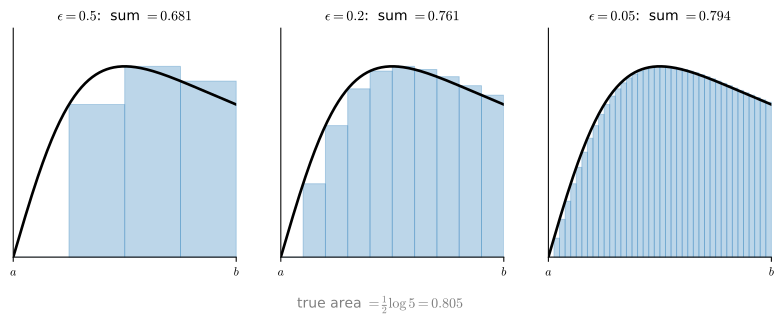
A bounded function \(f\) is Riemann integrable on \([a,b]\) if there is a number \(I\) such that every tagged sum approaches \(I\) as the partition mesh tends to zero:
\[ \int_a^b f(x)\,dx = I = \lim_{\|P\|\to0}\sum_{i=1}^N f(\xi_i)(x_i-x_{i-1}), \tag{25.4.1}\]
Here \(\|P\|=\max_i(x_i-x_{i-1})\), and the limit must be the same for every choice of tags. The integral is a continuous analogue of a sum; its variable is dummy, so \(\int_a^b f(x)\,dx=\int_a^b f(z)\,dz\). Bounded piecewise-continuous functions are Riemann integrable (Folland 1999), but this class does not cover every integral used in machine learning. Unbounded densities and infinite intervals require improper or Lebesgue integrals; the Riemann construction supplies the geometric starting point, while measure theory supplies the broader foundation. The integral it defines is monotone, so \(f \le g\) implies \(\int_a^b f\,dx \le \int_a^b g\,dx\), and additive over subintervals, so \(\int_a^c f\,dx = \int_a^b f\,dx + \int_b^c f\,dx\) for \(a\le b\le c\); both are plausible from the rectangle picture, and we use both below. (Some hypothesis on \(f\) is genuinely needed: for the function that is \(1\) on the rationals and \(0\) elsewhere, the rectangle sums never settle on any value at all. Lebesgue’s integral, built on measure theory rather than on slicing the axis, handles even that function, assigning it integral \(0\) because the rationals have measure zero. Probability theory uses this measure-theoretic extension when the Riemann conditions are insufficient.)
The definition does not yet provide a general evaluation method: rectangle sums can be computed by hand only for simple integrands such as \(\int_a^b x\,dx\). The next section develops a broader method. We first verify the convergence in Equation 25.4.1 numerically. Take \(\int_0^2 \tfrac{x}{1+x^2}\,dx\), whose exact value is \(\tfrac12\log 5\) (we will see why shortly), and refine the partition: the rectangle sum should approach the exact value, with error proportional to \(\epsilon\) for this left-endpoint rule.
import numpy as onp
def riemann(eps, a=0., b=2.):
    x = onp.arange(a, b, eps)
    return float(onp.sum(eps * x / (1 + x**2)))

truth = float(onp.log(onp.array(5.)) / 2)
for eps in [0.5, 0.1, 0.05, 0.01, 0.001]:
    approx = riemann(eps)
    print(f'eps={eps:<6} sum={approx:.6f}  error={abs(approx - truth):.6f}')
print(f'truth = (1/2) log 5 = {truth:.6f}')
eps=0.5 sum=0.680769 error=0.123950
eps=0.1 sum=0.783785 error=0.020934
eps=0.05 sum=0.794486 error=0.010233
eps=0.01 sum=0.802710 error=0.002009
eps=0.001 sum=0.804519 error=0.000200
truth = (1/2) log 5 = 0.804719The error falls by about a factor of ten each time we cut \(\epsilon\) by ten, confirming the first-order convergence of the left-rule. Refining the partition converges, but slowly, and does not produce a closed form.
25.4.2 The Fundamental Theorem of Calculus
Treating the upper limit as a variable connects integration to differentiation. Define the area-so-far function
\[ F(x) = \int_a^x f(y)\,dy, \tag{25.4.2}\]
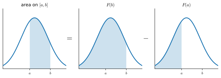
the signed area accumulated from the left endpoint \(a\) out to \(x\). This single function captures every definite integral at once: the area over any sub-interval is a difference of accumulated areas,
\[ \int_c^b f(x)\,dx = F(b) - F(c), \]
since the area out to \(b\) minus the area out to \(c\) leaves exactly the area between them. Figure 25.4.2 draws this subtraction, accumulating from a base point \(c\) at the left edge of the plot.
The function \(F\) encodes accumulated area. The fundamental theorem of calculus identifies the derivative of \(F\) and thereby provides an evaluation method.
Theorem (Fundamental theorem of calculus). Let \(f\) be continuous and let \(F(x)=\int_a^x f(y)\,dy\). Then \(F\) is differentiable and
\[ \frac{dF}{dx}(x) = f(x). \tag{25.4.3}\]
Proof. Differentiate \(F\) from the definition: nudge \(x\) by \(\epsilon\) and read off how much new area appears. By Equation 25.4.2 and additivity of the integral, the increment is a single thin sliver,
\[ F(x+\epsilon) - F(x) = \int_x^{x+\epsilon} f(y)\,dy . \]
The sliver sits over an interval of width \(\epsilon\). Write \(m_\epsilon = \inf_{[x,x+\epsilon]} f\) and \(M_\epsilon = \sup_{[x,x+\epsilon]} f\) for the tightest constant bounds on \(f\) there. Comparing \(f\) with those two constants, monotonicity of the integral pins the sliver between two rectangles of width \(\epsilon\):
\[ \epsilon\, m_\epsilon \ \le\ F(x+\epsilon) - F(x)\ \le\ \epsilon\, M_\epsilon . \]
Divide by \(\epsilon\). Because \(f\) is continuous at \(x\), for any \(\delta>0\) the whole interval \([x,x+\epsilon]\) eventually lies where \(|f(y)-f(x)|<\delta\), so \(m_\epsilon\) and \(M_\epsilon\) both converge to the single value \(f(x)\) as \(\epsilon \to 0\), and the squeeze forces \(\lim_{\epsilon\to 0}\frac{F(x+\epsilon)-F(x)}{\epsilon}=f(x)\) (for \(\epsilon<0\) the sliver sits to the left of \(x\) and the same bounds apply, with both sign flips canceling in the quotient). That limit is exactly \(F'(x)\). \(\blacksquare\)
The argument shows that the rate at which accumulated area grows is just the current height of the curve. This reverses the problem. Finding areas, hard on its own, becomes the search for an antiderivative, a function whose derivative is \(f\), which we can read straight off the derivative table of Section 25.1.2. If \(G'=f\) then \(G\) and \(F\) differ by a constant (they have the same derivative), and since that constant cancels in any difference,
\[ \int_a^b f(x)\,dx = G(b) - G(a) \tag{25.4.4}\]
for any antiderivative \(G\). The arbitrary constant of integration is real but irrelevant to definite integrals.
This converts the limit of sums into an antiderivative evaluation. The derivative of \(x^n\) is \(nx^{n-1}\), so running it backwards,
\[ \int_0^{x} n\,y^{n-1}\,dy = x^n - 0^n = x^n , \]
and since \(e^x\) is its own derivative,
\[ \int_0^{x} e^{t}\,dt = e^{x} - e^{0} = e^x - 1 . \]
Every integration rule is a differentiation rule read in reverse, which is why the running example obeyed \(\int_0^2 x/(1+x^2)\,dx=\tfrac12\log 5\): the antiderivative of \(x/(1+x^2)\) is \(\tfrac12\log(1+x^2)\), evaluated at the endpoints. Let us confirm the theorem numerically by checking that the area-so-far function \(F\) has derivative \(f\): compute \(F\) as a cumulative Riemann sum, finite-difference it, and compare against \(f\) itself.
import numpy as onp
f = lambda t: t / (1 + t**2)
G = lambda t: onp.log(1 + t**2) / 2          # antiderivative: F(x) = G(x) - G(0)
eps = 1e-3
x = onp.arange(0., 2., eps)
F = onp.cumsum(eps * f(x))                    # area-so-far via Riemann sum
dFdx = (F[1:] - F[:-1]) / eps                # telescopes to f(x[1:]) exactly
print('max |dF/dx - f|      :', float(onp.abs(dFdx - f(x[1:])).max()))
print('Riemann F(2) vs G(2)-G(0):', float(F[-1]), float(G(onp.array(2.))))
max |dF/dx - f| : 5.551115123125783e-14
Riemann F(2) vs G(2)-G(0): 0.8045188628837103 0.8047189562170501The first comparison is exact in exact arithmetic: differencing the cumulative sum telescopes, \(F(x+\epsilon)-F(x)\) collapsing back to the single term \(\epsilon f(x+\epsilon)\) that the sum just added. The printed error, a few parts in \(10^{5}\), is therefore not discretization error at all but pure float32 roundoff in the accumulated \(F\), amplified by the division by \(\epsilon\). The Riemann total \(F(2)\) agrees with the antiderivative value \(G(2)\) to about \(2\times 10^{-4}\), the expected first-order bias of the left-endpoint rule.
25.4.2.1 Improper Integrals
Many densities have an unbounded domain, including Gaussian, exponential, and heavy-tailed densities. Their normalization requires integration to infinity, whereas Equation 25.4.1 only defined integrals over a finite \([a,b]\). We fill the gap the same way we defined the integral itself: as a limit. The improper integral is
\[ \int_a^\infty f(x)\,dx = \lim_{b\to\infty}\int_a^b f(x)\,dx , \tag{25.4.5}\]
with \(\int_{-\infty}^\infty\) defined by splitting at any point and requiring both one-sided limits to exist on their own (a symmetric combination of the two is not enough). The limit may be finite, in which case the integral converges; otherwise it diverges, whether the partial integrals grow without bound or merely fail to settle. Whether the tail is “thin enough” is a genuine question. The test case is the power law \(x^{-p}\), for which the antiderivative gives
\[ \int_1^\infty x^{-p}\,dx = \lim_{b\to\infty}\frac{b^{1-p}-1}{1-p} = \begin{cases} \dfrac{1}{p-1}, & p>1\ \text{(converges)},\\[1ex] \infty, & p\le 1\ \text{(diverges)}.\end{cases} \]
The antiderivative \(\tfrac{b^{1-p}-1}{1-p}\) is the \(0/0\) indeterminate form at exactly \(p=1\), where the integrand \(x^{-1}\) has antiderivative \(\log x\) instead, so \(\int_1^\infty x^{-1}\,dx=\lim_{b\to\infty}\log b=\infty\); the case split above already records this divergent value. So \(\int_1^\infty x^{-2}\,dx = 1\) while \(\int_1^\infty x^{-1}\,dx=\infty\): the boundary between convergence and divergence sits exactly at \(p=1\). A heavy-tailed density is one whose tail decays like a power law rather than exponentially, and this single threshold is what decides whether such a density even has a finite normalizer or mean, a recurring concern once we reach probability. The following computation evaluates the convergent improper integral \(\int_0^\infty e^{-x}\,dx = 1\) in two ways: the exact partial integrals \(\int_0^b e^{-x}\,dx = 1-e^{-b}\), read off the antiderivative, and a left-Riemann approximation of each with \(\epsilon = 10^{-3}\).
import numpy as onp
for b in [1., 2., 5., 10., 20.]:
    x = onp.arange(0., b, 1e-3)
    left = float(onp.sum(1e-3 * onp.exp(-x)))
    exact = 1 - float(onp.exp(onp.array(-b)))
    print(f'b={b:<4}  left-Riemann sum={left:.6f}  exact 1-e^-b={exact:.6f}')
b=1.0 left-Riemann sum=0.632437 exact 1-e^-b=0.632121
b=2.0 left-Riemann sum=0.865097 exact 1-e^-b=0.864665
b=5.0 left-Riemann sum=0.993759 exact 1-e^-b=0.993262
b=10.0 left-Riemann sum=1.000455 exact 1-e^-b=0.999955
b=20.0 left-Riemann sum=1.000500 exact 1-e^-b=1.000000The two columns isolate different error sources. The exact partials approach \(1\) quickly: the truncation error of stopping at \(b\) is \(e^{-b}\), already invisible at six decimals by \(b=20\). The left-Riemann column tells a subtler story: it overshoots and settles near \(1.0005\), not \(1\). That residue is discretization error. The left rule samples each slice at its left edge, where the decreasing integrand \(e^{-x}\) is largest, so every rectangle overcounts slightly; the overcounts add up to a bias of \(\approx \tfrac{\epsilon}{2}\bigl(f(0)-f(b)\bigr) \to \tfrac{\epsilon}{2} = 0.0005\). The two errors are independent: increasing \(b\) reduces truncation error, while shrinking \(\epsilon\) reduces discretization error. Changing either parameter does not eliminate the other error.
25.4.2.2 Integration by Parts
The fundamental theorem turns every differentiation rule into an integration rule. Converted, the product rule becomes integration by parts.
Proposition (Integration by parts). For continuously differentiable \(u\) and \(v\) on \([a,b]\),
\[ \int_a^b u(x)\,v'(x)\,dx = \Bigl[\,u(x)\,v(x)\,\Bigr]_a^b - \int_a^b u'(x)\,v(x)\,dx , \tag{25.4.6}\]
where \([\,h(x)\,]_a^b\) abbreviates \(h(b)-h(a)\).
Proof. By the product rule, \(uv\) is an antiderivative of \(u'v + uv'\), so Equation 25.4.4 gives \(\int_a^b (u'v + uv')\,dx = [\,u(x)v(x)\,]_a^b\); subtract \(\int_a^b u'v\,dx\) from both sides. \(\blacksquare\)
The formula transfers the derivative from one factor to the other. It is useful when the new integrand \(u'v\) is simpler than the old one \(uv'\). The model example takes \(u(x)=x\) and \(v'(x)=e^{-x}\), so that \(u'=1\) and \(v=-e^{-x}\): applying Equation 25.4.6 on \([0,b]\) and letting \(b\to\infty\),
\[ \int_0^\infty x\,e^{-x}\,dx = \Bigl[\,-x\,e^{-x}\,\Bigr]_0^\infty + \int_0^\infty e^{-x}\,dx = 0 + 1 = 1 . \]
The boundary term vanishes because \(x e^{-x}\to 0\) at both ends, and what survives is exactly the improper integral computed above. This particular value is the mean of the exponential distribution (Section 27.2), and it illustrates how the identity is used throughout probability: expectations \(\int g(x)\,p(x)\,dx\) are integrals of products, and often the only move available is to shift a derivative from a factor we cannot handle onto one we can. The identity returns in Hyvärinen’s score matching (Hyvärinen 2005) (Section 29.4), where one integration by parts converts an objective involving an unknown score into one that can be estimated from samples. The unavailable quantity is the score of the data distribution, the gradient \(\nabla_{\mathbf{x}} \log p(\mathbf{x})\) of the log-density with respect to the data point.
25.4.2.3 A Note on Signed Area
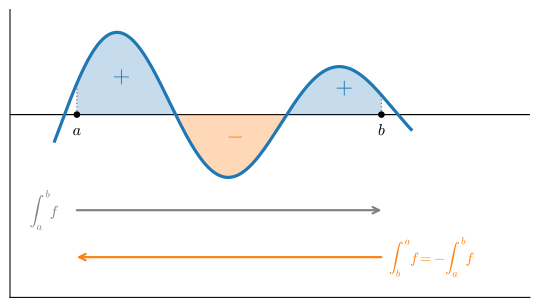
The evaluation rule Equation 25.4.4 produces negative numbers, which can be jarring if “area” is supposed to be positive. The resolution is that integrals measure signed area, governed by two independent sign rules. First, where \(f<0\) the area counts as negative: \(\int_0^1 (-1)\,dx = -1\). Second, integrating right-to-left negates the result: \(\int_b^a f = -\int_a^b f\). Each flip, reflecting across the \(x\)-axis or reversing the limits, introduces one minus sign; Figure 25.4.3 shows both rules on one curve. Apply them in turn to a single example: \(\int_0^{-1} 1\,dx = -1\) (one flip, from reversed limits), while \(\int_0^{-1}(-1)\,dx = 1\) (two flips, which cancel). This is the same signed-area convention the determinant followed for transformed regions in Section 24.1, and it is exactly what makes the change-of-variables formula below come out right.
25.4.3 Change of Variables
Every differentiation rule has an integration counterpart obtained by running the fundamental theorem backwards: the sum rule gives linearity, the product rule gave us integration by parts (Section 25.4.2.2), and the chain rule, most useful of all for us, gives the change-of-variables formula: the substitution rule that evaluates many integrals the derivative table alone cannot. The next section carries it into higher dimensions.
Suppose we reparametrize the variable through a function \(u\). The chain rule says \(\frac{d}{dx}F(u(x)) = F'(u(x))\,u'(x)\); feeding this through the fundamental theorem with \(F'=f\) and integrating both sides yields the change-of-variables formula
\[ \int_{u(a)}^{u(b)} f(y)\,dy = \int_a^b f(u(x))\,\frac{du}{dx}\,dx . \tag{25.4.7}\]
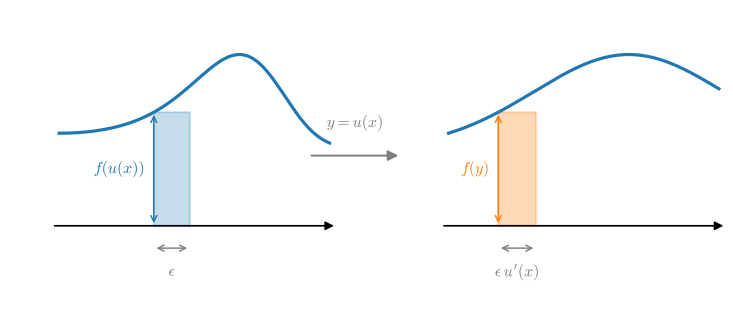
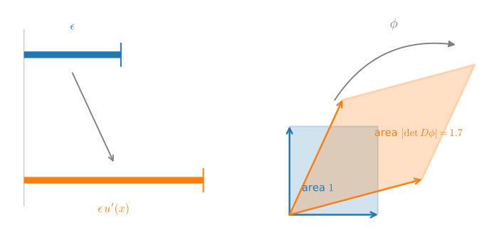
A thin rectangle explains the factor \(\frac{du}{dx}\). On the left side of Equation 25.4.7, the sliver from \(x\) to \(x+\epsilon\) has area \(\approx \epsilon\,f(u(x))\). On the right, the corresponding sliver runs from \(u(x)\) to \(u(x+\epsilon)\approx u(x)+\epsilon\,u'(x)\), so its width is stretched by the factor \(u'(x)\) and its area is \(\approx \epsilon\,u'(x)\,f(u(x))\). To make the two slivers agree we must multiply by exactly the local stretch \(\frac{du}{dx}\), as Figure 25.4.4 shows.
A suitable \(u\) reduces the original integral to a known form. Taking \(f=1\) and \(u(x)=e^{-x^2}\) (so \(u'(x)=-2x\,e^{-x^2}\)),
\[ e^{-1}-1 = \int_{e^{0}}^{e^{-1}} 1\,dy = -2\int_0^{1} x\,e^{-x^2}\,dx \quad\Longrightarrow\quad \int_0^{1} x\,e^{-x^2}\,dx = \frac{1-e^{-1}}{2}, \]
a closed form that no amount of rectangle-summing would have revealed. (Keep the two variables apart: \(y\) is the transformed variable on the left of Equation 25.4.7, \(x\) the original one on the right; the result is a statement about the \(x\)-integral.)
25.4.4 Multiple Integrals
In one dimension the integral was a limit of rectangle sums, and nothing in that recipe was attached to the line. This section runs the same recipe over regions of \(\mathbb{R}^n\), establishes Fubini’s theorem, which reduces such integrals to iterated one-dimensional ones, and lifts the change-of-variables rule to \(n\) dimensions.
25.4.4.1 Double Integrals
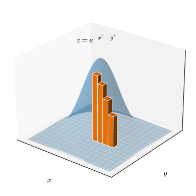
In higher dimensions we integrate over regions. For \(f(x,y)\) on a rectangle \(U=[a,b]\times[c,d]\), the integral is the (signed) volume trapped between the surface \(z=f(x,y)\) and the base plane, written \(\int_U f(x,y)\,dx\,dy\). The Riemann approximation tiles \(U\) with \(\epsilon\times\epsilon\) squares and sums boxes with height \(f\). Figure 25.4.5 shows our running example, the two-dimensional bell \(e^{-x^2-y^2}\) over the box \([-2,2]^2\); the cell totals its boxes.
import math
import numpy as onp
eps = 1e-2
x, y = onp.meshgrid(onp.arange(-2., 2., eps), onp.arange(-2., 2., eps),
                   indexing='ij')
vol = float(onp.sum(eps ** 2 * onp.exp(-x**2 - y**2)))
exact = math.pi * math.erf(2.) ** 2
print(f'Riemann volume over the box [-2, 2]^2 : {vol:.5f}')
print(f'exact volume  pi * erf(2)^2           : {exact:.5f}')
Riemann volume over the box [-2, 2]^2 : 3.11227
exact volume pi * erf(2)^2 : 3.11227The exact value involves the error function \(\operatorname{erf}(z)=\tfrac{2}{\sqrt{\pi}}\int_0^z e^{-t^2}\,dt\), the Gaussian’s antiderivative, suitably normalized. It has no elementary formula, but the library provides it as a built-in, which is how the cell computes the exact volume \(\pi\operatorname{erf}(2)^2\) (an expression derived at the end of this section, where the Gaussian integral is evaluated).
25.4.4.2 Fubini’s Theorem
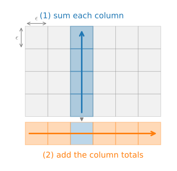
How do we get from grid sums back to the fundamental theorem? Discretize the region into \(\epsilon\times \epsilon\) squares indexed by integers \(i,j\); the integral is approximately \(\sum_{i,j}\epsilon^2 f(\epsilon i, \epsilon j)\). This is just a sum of numbers on a grid, and a finite sum can be totalled in any order. Summing columns-first (add up each column \(i\), then add the column totals) we get
\[ \sum_j \epsilon\!\left(\sum_i \epsilon\, f(\epsilon i, \epsilon j)\right), \]
illustrated in Figure 25.4.6. The inner sum is the Riemann discretization of \(\int_a^b f(x,\epsilon j)\,dx\), and the outer sum then integrates that over \(y\).
For the finite grid sums the reordering is trivial, and that triviality carries none of the theorem’s content: the integral is the limit of the grid sums, and the substance is that the interchange survives the two limiting processes. That step we take on faith. Fubini’s theorem (Folland 1999) requires \(f\) to be absolutely integrable, meaning
\[ \int_U |f(x,y)|\,dx\,dy < \infty , \]
and concludes that the double integral equals either iterated integral,
\[ \int_U f(x,y)\,dx\,dy = \int_c^{d}\!\left(\int_a^{b} f(x,y)\,dx\right)dy = \int_a^{b}\!\left(\int_c^{d} f(x,y)\,dy\right)dx . \tag{25.4.8}\]
The hypothesis matters. The standard counterexample is \(f(x,y)=(x^2-y^2)/(x^2+y^2)^2\) on \([0,1]^2\): integrating \(x\) first gives \(-\tfrac{\pi}{4}\), integrating \(y\) first gives \(+\tfrac{\pi}{4}\), and the orders disagree precisely because the singularity at the origin makes \(\int_U |f|\,dx\,dy\) infinite. For the continuous, absolutely integrable functions of machine learning the absolute-integrability condition holds, so either integration order is valid. When the region \(U\) is more complicated than a rectangle we write the integral compactly as \(\int_U f(\mathbf{x})\,d\mathbf{x}\); it is defined by zero-extension: extend \(f\) by \(0\) outside \(U\) and integrate the extended function over any rectangle containing \(U\).
25.4.4.3 Change of Variables in Many Dimensions
The one-dimensional stretch factor \(du/dx\) becomes a local volume factor in several dimensions. This factor will let polar coordinates separate the Gaussian integral below. Let \(U\subseteq\mathbb{R}^n\) be open and let \(\boldsymbol{\phi}:U\to\mathbb{R}^n\) be a \(C^1\)-diffeomorphism onto its image; that is, \(\boldsymbol{\phi}\) is continuously differentiable, injective, and has \(\det D\boldsymbol{\phi}(\mathbf{x})\neq 0\) everywhere on \(U\). (Injectivity stops the map folding space onto itself; the nonvanishing Jacobian keeps it from collapsing a region to lower dimension, and together they make \(\boldsymbol{\phi}\) invertible on \(\boldsymbol{\phi}(U)\) with a \(C^1\) inverse.) Then, for absolutely integrable \(f\) (again, \(\int |f|\,d\mathbf{x} < \infty\)), a theorem we also take on faith (Folland 1999) states that
\[ \int_{\boldsymbol{\phi}(U)} f(\mathbf{x})\,d\mathbf{x} = \int_{U} f(\boldsymbol{\phi}(\mathbf{x}))\, \bigl|\det D\boldsymbol{\phi}(\mathbf{x})\bigr|\,d\mathbf{x}, \tag{25.4.9}\]
where \(D\boldsymbol{\phi}\) is the Jacobian of \(\boldsymbol{\phi}\), the matrix of partial derivatives introduced in Section 25.3.1.
Compare Equation 25.4.9 with the one-dimensional rule Equation 25.4.7: the scalar stretch \(\frac{du}{dx}\) has been replaced by \(|\det D\boldsymbol{\phi}|\), and the determinant of a linear map is exactly the factor by which it scales area or volume, the signed-area reading of the determinant from Section 24.1. So a tiny cube of volume \(d\mathbf{x}\) is sent to a tiny parallelepiped of volume \(|\det D\boldsymbol{\phi}|\,d\mathbf{x}\), and the factor in the integrand compensates for exactly that distortion. Figure 25.4.7 puts the one- and two-dimensional pictures side by side.
Equation Equation 25.4.9 is a statement about area and volume: it says how the integral of a fixed function transports under a reparametrization of the domain. Apply it instead to a probability density, a function that must keep integrating to \(1\), and the very same Jacobian factor becomes the change-of-variables-for-densities rule of Section 27.1, whose \(-\log|\det D\boldsymbol{\phi}|\) correction is the exact mechanism behind normalizing flows (Section 29.1.5). We state the area theorem here and defer that density specialization to the probability chapter.
25.4.4.4 The Gaussian Integral
The preceding results evaluate the Gaussian integral, which we will meet again as the normalizer of the normal distribution. It is the one-dimensional integral
\[ \int_{-\infty}^{\infty} e^{-x^2}\,dx \]
that resists direct attack: \(e^{-x^2}\) has no elementary antiderivative (its antiderivative is the error function from the bell-volume cell, defined as that integral rather than expressed in older functions), so the fundamental theorem does not apply directly. The standard derivation introduces a second dimension.
One preliminary. The plan involves integrals over all of \(\mathbb{R}^2\), and we have defined improper integrals only on the line Equation 25.4.5. For a nonnegative integrand the same limiting idea works in any dimension, by exhaustion: define \(\iint_{\mathbb{R}^2} f\,dx\,dy\) as the limit of the integrals over the growing boxes \([-b,b]^2\) as \(b\to\infty\). Because \(f\ge 0\), these integrals can only increase as the box grows, so the limit exists (it may be \(+\infty\)), and exhausting the plane by discs or any other expanding family of regions gives the same value, since every disc is contained in some box and every box in some disc. Everything we integrate below is nonnegative, so this definition is in force throughout.
Square the integral and use a different dummy variable in the second factor:
\[ \left(\int_{-\infty}^{\infty} e^{-x^2}\,dx\right)^{\!2} = \int_{-\infty}^{\infty} e^{-x^2}\,dx \int_{-\infty}^{\infty} e^{-y^2}\,dy = \int_{-\infty}^{\infty}\!\!\int_{-\infty}^{\infty} e^{-x^2-y^2}\,dx\,dy . \tag{25.4.10}\]
The second equality says that the iterated integral equals the double integral over the whole plane: this is Fubini’s theorem again, now on \(\mathbb{R}^2\) rather than on a rectangle, and we grant this whole-plane form on the same authority (Folland 1999).
The two-dimensional integral has something its one-dimensional parent lacked, rotational symmetry, and polar coordinates \(\boldsymbol{\phi}(r,\theta)=(r\cos\theta, r\sin\theta)\) are built to exploit it. Take the open set \(U=(0,\infty)\times(0,2\pi)\). On \(U\) the map \(\boldsymbol{\phi}\) is injective, and its Jacobian determinant
\[ \bigl|\det D\boldsymbol{\phi}\bigr| = \left|\det\begin{bmatrix}\cos\theta & -r\sin\theta\\ \sin\theta & r\cos\theta\end{bmatrix}\right| = r(\cos^2\theta + \sin^2\theta) = r \]
is nonzero there, so \(\boldsymbol{\phi}\) is a \(C^1\)-diffeomorphism of \(U\) onto its image. That image is not quite the whole plane: \(\boldsymbol{\phi}(U)\) is \(\mathbb{R}^2\) minus the ray \(\{(x, 0) : x \ge 0\}\), the points the excluded angle \(\theta = 0\) would have produced. A ray, however, has measure zero: it can be covered by rectangles of arbitrarily small total area (a notion Section 27.1 returns to), and we grant, once more from the same source (Folland 1999), that a set of measure zero contributes nothing to any integral. Integrating over \(\boldsymbol{\phi}(U)\) is therefore the same as integrating over the plane, and the change of variables Equation 25.4.9 on \(U\) hands the integrand the factor \(r\) that makes it elementary:
\[ \iint_{\mathbb{R}^2} e^{-x^2-y^2}\,dx\,dy = \int_{\boldsymbol{\phi}(U)} e^{-x^2-y^2}\,dx\,dy = \int_0^\infty\!\!\int_0^{2\pi} r\,e^{-r^2}\,d\theta\,dr = 2\pi\int_0^\infty r\,e^{-r^2}\,dr = \pi , \]
the last step because \(-\tfrac12 e^{-r^2}\) is an antiderivative of \(r\,e^{-r^2}\), so the improper integral is \(\tfrac12\). (Strictly, one applies Equation 25.4.9 on the bounded sets \(U_b=(0,b)\times(0,2\pi)\), where the continuous bounded integrand is certainly absolutely integrable, and lets \(b\to\infty\); both sides increase to the values shown.) Taking the square root of Equation 25.4.10 (the positive one, since the integrand is positive) gives
\[ \int_{-\infty}^{\infty} e^{-x^2}\,dx = \sqrt{\pi} . \]
The same factorization also explains the bell-volume cell’s exact value: over the box, \(\bigl(\int_{-2}^{2} e^{-x^2}\,dx\bigr)^2 = \bigl(\sqrt{\pi}\,\operatorname{erf}(2)\bigr)^2 = \pi\operatorname{erf}(2)^2 \approx 3.11227\), shy of the full-plane \(\pi\) by exactly the truncated tails. The cell verifies the two-dimensional integral numerically by summing the integrand over a fine grid on \([-6,6]^2\), a box wide enough that the Gaussian’s tails beyond it contribute nothing to six decimals.
import numpy as onp
g = onp.arange(-6., 6., 0.01)
x, y = onp.meshgrid(g, g, indexing='ij')
val = float(onp.sum(0.01 ** 2 * onp.exp(-x**2 - y**2)))
print('grid integral of e^(-x^2-y^2):', round(val, 6))
print('exact value pi               :', round(float(onp.pi), 6))
grid integral of e^(-x^2-y^2): 3.141593
exact value pi : 3.14159325.4.5 Integration in Probability
This is why a deep-learning reader needs integration at all. A continuous probability density is nothing more than a non-negative function that is normalized, meaning its total integral is \(1\):
\[ p(x)\ge 0, \qquad \int_{\mathcal X} p(x)\,dx = 1 . \tag{25.4.11}\]
The Gaussian integral above is precisely what supplies the normalizer: we showed \(\int_{-\infty}^\infty e^{-x^2}\,dx=\sqrt\pi\), so the function \(p(x)=\tfrac{1}{\sqrt\pi}e^{-x^2}\) integrates to \(1\) and is a bona fide density. An expectation is then an integral average, weighting each value by its density,
\[ \mathbb{E}[X] = \int_{\mathcal X} x\,p(x)\,dx, \qquad \mathbb{E}[g(X)] = \int_{\mathcal X} g(x)\,p(x)\,dx . \tag{25.4.12}\]
In several variables a joint density satisfies \(\iint p(x,y)\,dx\,dy = 1\), and marginals are obtained by integrating a variable out, \(p(x)=\int p(x,y)\,dy\); Fubini Equation 25.4.8 guarantees the order of integration does not matter (densities are absolutely integrable, so the caveat above never bites). The cell verifies that \(\tfrac{1}{\sqrt\pi}e^{-x^2}\) is normalized and computes its mean, which symmetry sends to \(0\).
import numpy as onp
x = onp.arange(-8., 8., 1e-3)
p = onp.exp(-x**2) / onp.sqrt(onp.array(onp.pi))
print('total mass  integral p dx :', round(float(onp.sum(1e-3 * p)), 6))
print('mean integral x p dx:', round(float(onp.sum(1e-3 * x * p)), 6))total mass integral p dx : 1.0
mean integral x p dx: 0.0total mass integral p dx : 1.0
mean integral x p dx: 0.0total mass integral p dx : 1.0
mean integral x p dx: 0.0total mass integral p dx : 1.0
mean integral x p dx: -0.0When an expectation has no closed form, the rule rather than the exception in deep learning, we estimate it by Monte Carlo (Metropolis and Ulam 1949): draw samples \(x_i\sim p\) and average,
\[ \mathbb{E}[g(X)] \approx \frac{1}{n}\sum_{i=1}^n g(x_i), \tag{25.4.13}\]
a stochastic counterpart of the Riemann sum that ignores the geometry of the domain. The law of large numbers (Section 27.5) guarantees that it works: the sample average converges to the true expectation. The error scale comes from a variance computation: the estimator’s standard deviation is \(\mathrm{sd}(g(X))/\sqrt{n}\), an order-\(1/\sqrt{n}\) error whose limiting distribution comes from the central limit theorem (Section 27.2). The rate depends only on the sample size \(n\), not on the dimension. (The fine print: the constant in front of \(1/\sqrt{n}\) is the standard deviation of \(g(X)\), and that can grow with the dimension; what is dimension-free is the exponent, and it is the exponent that grids lose.) That dimension-free rate is decisive. A grid laid down to resolution \(\epsilon\) in \(d\) dimensions costs \(N=\epsilon^{-d}\) evaluations. The left rule we have used throughout has error \(\propto\epsilon\), so it achieves only \(N^{-1/d}\); even a second-order rule (the midpoint rule, which samples each slice at its center, or the trapezoid rule, which averages the two edge heights) has error \(\propto\epsilon^2\) and manages just \(N^{-2/d}\). Either way the exponent is divided by the dimension, the curse of dimensionality, while Monte Carlo keeps its \(N^{-1/2}\) in every dimension. This is why sampling, rather than grid quadrature, is how expectations are computed at scale. The sample-mean estimator and its \(\sigma^2/n\) variance return with random variables (Section 27.1), and the law of large numbers behind the guarantee is stated in Section 27.5. The cell makes this concrete: it estimates \(\int_0^1 e^{-x^2}\,dx\) by averaging \(e^{-x_i^2}\) over uniform samples, prints the running estimate against a midpoint quadrature fine enough to be exact at the printed precision, and then plots the measured error of the running estimate against the sample size on log-log axes, next to the predicted guide line \(0.2\,N^{-1/2}\) (the constant \(0.2\) is \(\mathrm{sd}(e^{-X^2})\) for uniform \(X\)).
np.random.seed(1)
# E[e^{-X^2}], X ~ U[0, 1], by Monte Carlo vs a fine midpoint quadrature
# (midpoint is second-order: at eps=1e-4 its bias ~ 3e-10, below the print).
quad = float(np.sum(1e-4 * np.exp(-(np.arange(0., 1., 1e-4) + 5e-5) ** 2)))
draws = np.exp(-np.random.rand(100000) ** 2)
running = np.cumsum(draws) / np.arange(1., 100001.)   # running MC estimate
for n in [10, 100, 1000, 10000, 100000]:
    mc = float(running[n - 1])
    print(f'n={n:<7} Monte Carlo={mc:.5f}  error={abs(mc - quad):.1e}')
print(f'midpoint quadrature  ={quad:.5f}')

# Measured error of the running estimate vs the predicted sd(g)/sqrt(N)
# line, sampled at log-spaced N so the log-log plot stays light.
Ns = np.logspace(1., 5., 201)
err = np.abs(running[Ns.astype('int32') - 1] - quad)
d2l.plot(Ns, [err, 0.2 * Ns ** -0.5], 'samples N', 'integration error',
         xscale='log', yscale='log',
legend=['measured MC error', '$0.2\\,N^{-1/2}$ guide'])n=10 Monte Carlo=0.87741 error=1.3e-01
n=100 Monte Carlo=0.75454 error=7.7e-03
n=1000 Monte Carlo=0.74619 error=6.3e-04
n=10000 Monte Carlo=0.74833 error=1.5e-03
n=100000 Monte Carlo=0.74719 error=3.7e-04
midpoint quadrature =0.74682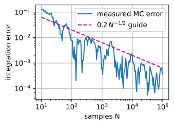
n=10      Monte Carlo=0.87741  error=1.3e-01
n=100     Monte Carlo=0.75454  error=7.7e-03
n=1000    Monte Carlo=0.74619  error=6.3e-04
n=10000   Monte Carlo=0.74833  error=1.5e-03
n=100000  Monte Carlo=0.74719  error=3.7e-04
midpoint quadrature  =0.74682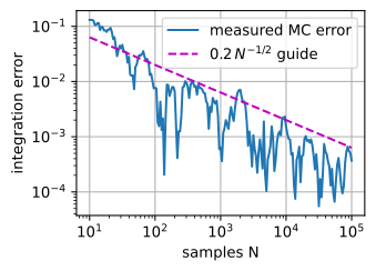
n=10      Monte Carlo=0.87741  error=1.3e-01
n=100     Monte Carlo=0.75454  error=7.7e-03
n=1000    Monte Carlo=0.74619  error=6.3e-04
n=10000   Monte Carlo=0.74833  error=1.5e-03
n=100000  Monte Carlo=0.74719  error=3.7e-04
midpoint quadrature  =0.74682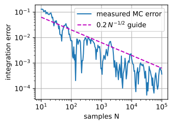
n=10      Monte Carlo=0.77087  error=2.4e-02
n=100     Monte Carlo=0.76334  error=1.7e-02
n=1000    Monte Carlo=0.75395  error=7.1e-03
n=10000   Monte Carlo=0.74625  error=5.7e-04
n=100000  Monte Carlo=0.74693  error=1.0e-04
midpoint quadrature  =0.74682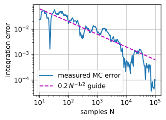
The running estimate closes in on the quadrature value as \(n\) grows, unevenly, as randomness must: the \(1/\sqrt{n}\) rate holds in expectation (about \(6\times 10^{-4}\) at \(n=10^5\) for this integrand), and an individual prefix can have unusually small error, as the \(n=1000\) row here does, with error a tenth of the predicted scale. The log-log plot shows the measured error scattering around the \(0.2\,N^{-1/2}\) guide line while tracking its slope of \(-\tfrac12\) across four decades. A second-order grid would beat that slope at \(d=2\) (error \(N^{-1}\)), tie it exactly at \(d=4\) (\(N^{-2/4}=N^{-1/2}\)), and by \(d=6\) and \(d=10\) flatten to slopes \(-\tfrac13\) and \(-\tfrac15\) and lose badly; for the first-order left rule the break-even is already \(d=2\). Past a handful of dimensions, sampling is the only practical choice, which is the quantitative face of the curse of dimensionality.
25.4.5.1 Differentiating under the Integral Sign
NoteAssumptions behind common calculus interchanges
Several formulas in this appendix are conditional statements. The following sufficient conditions cover the cases used most often in machine learning:
- A derivative or Jacobian formula assumes differentiability on a neighborhood of the point. At a ReLU kink, autograd returns a library convention rather than a classical derivative.
- Equality of mixed partials and symmetry of the Hessian follow when the second partial derivatives are continuous on a neighborhood.
- Swapping two integrals is valid for a non-negative integrand (Tonelli) or an absolutely integrable one (Fubini). Conditional convergence needs separate care.
- Passing a limit or derivative through an integral is justified when an integrable dominating function controls the relevant sequence or derivative throughout a neighborhood of the parameter. Moving boundaries contribute the Leibniz boundary terms below.
- A change of variables requires a one-to-one differentiable map on the region of interest, or a partition into such regions, and a nonzero Jacobian determinant away from negligible boundary sets.
These are convenient sufficient conditions, not the weakest possible ones. When a model changes support, approaches a singular distribution, or contains a nonsmooth branch, pause and check the relevant theorem rather than applying the formal rule mechanically.
One more interchange matters in deep learning: moving a gradient through an integral. When an integrand depends on a parameter \(\boldsymbol{\theta}\), we will routinely write
\[ \nabla_{\boldsymbol{\theta}} \int f(x, \boldsymbol{\theta})\,dx = \int \nabla_{\boldsymbol{\theta}} f(x, \boldsymbol{\theta})\,dx . \]
The swap needs a hypothesis. The standard sufficient condition is that, near the current \(\boldsymbol{\theta}\), the integrands’ derivatives are bounded in magnitude by a single integrable function of \(x\); it follows from the dominated convergence theorem, which we also state on faith (Folland 1999). Many smooth, rapidly decaying densities used in deep learning comply, but the condition must be checked rather than inferred from smoothness alone. Moving support and increasingly sharp parameter-dependent spikes are two common ways it can fail; failure is not limited to those cases.
When it is the limits of integration that move, the correct derivative is known in closed form. The Leibniz rule (Folland 1999) states that
\[ \frac{d}{d\theta} \int_{a(\theta)}^{b(\theta)} f(x, \theta)\,dx = \int_{a(\theta)}^{b(\theta)} \frac{\partial f}{\partial\theta}(x,\theta)\,dx + f\bigl(b(\theta), \theta\bigr)\,b'(\theta) - f\bigl(a(\theta), \theta\bigr)\,a'(\theta) . \]
The two boundary terms are precisely what the naive swap forgets: each moving endpoint sweeps area in or out at the rate the limit moves, weighted by the integrand’s value there. A density supported on \([0, \theta]\) is the classic trap: dropping the boundary term produces a confidently wrong gradient.
Two results we lean on later are direct applications of this swap. Differentiating the normalization \(\int p_{\boldsymbol{\theta}}(x)\,dx = 1\) under the integral shows the score \(\nabla_{\boldsymbol{\theta}}\log p_{\boldsymbol{\theta}}\) has mean zero, the seed of Fisher information (Section 27.3). This score is a gradient with respect to the parameters \(\boldsymbol{\theta}\); it is a different object from the data score \(\nabla_{\mathbf{x}}\log p(\mathbf{x})\) that score matching estimates, which is a gradient with respect to the data point. Applying the same swap to an expectation gives, when \(g\) itself does not depend on \(\boldsymbol\theta\),
\[ \nabla_{\boldsymbol{\theta}}\,\mathbb{E}_{x\sim p_{\boldsymbol{\theta}}}[g(x)] = \mathbb{E}\bigl[g(x)\,\nabla_{\boldsymbol{\theta}}\log p_{\boldsymbol{\theta}}(x)\bigr]. \tag{25.4.14}\]
This is the score-function, or REINFORCE, identity (Williams 1992), at the heart of policy-gradient methods. If \(g(x,\boldsymbol\theta)\) also depends directly on the parameter, add the ordinary term \(\mathbb E[\nabla_{\boldsymbol\theta}g(x,\boldsymbol\theta)]\) to the right.
25.4.5.1.1 Pathwise and Score-Function Gradients
The score-function identity is only one way to differentiate an expectation. If a random variable can be generated by transforming parameter-free noise,
\[ \boldsymbol\epsilon\sim q,\qquad x=T_{\boldsymbol\theta}(\boldsymbol\epsilon), \]
then
\[ \nabla_{\boldsymbol\theta} \mathbb E_{x\sim p_{\boldsymbol\theta}}[g(x,\boldsymbol\theta)] = \mathbb E_{\boldsymbol\epsilon\sim q} \left[\frac{d}{d\boldsymbol\theta} g(T_{\boldsymbol\theta}(\boldsymbol\epsilon),\boldsymbol\theta)\right]. \tag{25.4.15}\]
This is the pathwise, or reparameterization, gradient. For example, \(X\sim\mathcal N(\mu,\sigma^2)\) can be written \(X=\mu+\sigma\epsilon\) with \(\epsilon\sim\mathcal N(0,1)\); automatic differentiation then follows an ordinary differentiable path from \(\mu\) and \(\sigma\) to the sample. Variational autoencoders use exactly this device to backpropagate through a Gaussian latent variable.
The two estimators are both Monte Carlo estimators of the same derivative, but their variances can differ sharply. For \(L(\theta)=\mathbb E_{X\sim\mathcal N(\theta,1)}[X^2]=\theta^2+1\), the true derivative is \(2\theta\). With \(X=\theta+\epsilon\), one sample contributes \(2X\) to the pathwise estimator. The score of the normal location family is \(\partial_\theta\log p_\theta(X)=X-\theta=\epsilon\), so REINFORCE contributes \(X^2\epsilon\). Subtracting any baseline \(b\) that does not depend on \(X\) leaves the expectation unchanged because \(\mathbb E[\epsilon]=0\); choosing a good baseline can remove substantial variance.
import numpy as onp
rng = onp.random.default_rng(7)
theta, n = 1.5, 200000
eps = rng.standard_normal(n)
x = theta + eps
pathwise = 2 * x
score = x**2 * eps
b_opt = theta**2 + 3                         # minimizes Var[(X^2-b) epsilon]
score_baseline = (x**2 - b_opt) * eps

def report(name, samples):
    se = samples.std(ddof=1) / onp.sqrt(len(samples))
    print(f'{name:22s} mean={samples.mean():.4f}  '
          f'sample sd={samples.std(ddof=1):.3f}  MC se={se:.4f}')

print(f'true derivative = {2 * theta:.4f}')
report('pathwise', pathwise)
report('score function', score)
report('score + baseline', score_baseline)
true derivative = 3.0000
pathwise mean=3.0019 sample sd=1.998 MC se=0.0045
score function mean=2.9974 sample sd=7.162 MC se=0.0160
score + baseline mean=2.9924 sample sd=4.878 MC se=0.0109All three sample means agree with \(2\theta\) within Monte Carlo error. The pathwise estimate is much less noisy on this smooth problem; the baseline helps REINFORCE but does not generally close the gap. This is a common pattern, not a universal ordering: variance depends on the model, transformation, and integrand.
The score estimator remains valuable because it does not differentiate through the sampled value. It therefore works for Bernoulli and categorical choices, where an exact differentiable reparameterization is generally unavailable. Continuous relaxations such as Gumbel–softmax (Jang et al. 2017; Maddison et al. 2017) create a differentiable surrogate; straight-through estimators use a discrete forward value and a surrogate backward derivative. These can reduce variance, but they are biased for the original discrete objective unless a separate argument establishes otherwise.
Both identities inherit the assumptions of differentiation under the integral sign. The score form also assumes the relevant support does not move with \(\boldsymbol\theta\), or that the missing boundary terms are included. The pathwise form requires a differentiable transformation and an integrable bound for its derivative. In practice, “differentiate through randomness” therefore means choosing an estimator, checking its assumptions, and reporting its variance or Monte Carlo standard error—not merely asking an autodiff library for a gradient.
25.4.6 Summary
- The definite integral \(\int_a^b f\,dx\) is the limit of Riemann rectangle sums Equation 25.4.1: the signed area under \(f\), with negative contributions where \(f<0\) or when the limits run backwards.
- The fundamental theorem of calculus Equation 25.4.3 says the area-so-far function \(F(x)=\int_a^x f\) has derivative \(F'=f\). Integration is therefore differentiation reversed: \(\int_a^b f = G(b)-G(a)\) for any antiderivative \(G\).
- Improper integrals extend the definition to infinite domains as a limit; \(\int_1^\infty x^{-p}\,dx\) converges exactly when \(p>1\).
- Integration by parts Equation 25.4.6 converts \(\int u\,v'\) into a boundary term minus \(\int u'\,v\): the product rule run backwards, and the standard device for moving a derivative onto the factor that can absorb it (score matching, expectations of products).
- Change of variables multiplies by the local stretch: \(du/dx\) in one dimension Equation 25.4.7, the Jacobian determinant \(|\det D\boldsymbol{\phi}|\) for a \(C^1\)-diffeomorphism in many Equation 25.4.9, the same volume-scaling read off the determinant.
- Fubini’s theorem evaluates a multiple integral as iterated single integrals in either order, for absolutely integrable functions (\(\int_U |f|\,d\mathbf{x} < \infty\)).
- Integration is the language of continuous probability: a density is a normalized non-negative function \(\int p = 1\), and an expectation is the integral \(\int x\,p\,dx\). When it has no closed form, Monte Carlo estimates it by sampling, converging at the dimension-free rate \(1/\sqrt{n}\), unlike a grid, whose cost explodes with dimension.
- Gradients of expectations admit two principal Monte Carlo estimators. The score-function estimator differentiates the log-density and works for discrete samples but can have high variance; the pathwise estimator differentiates a transformation of parameter-free noise and is usually preferred when such a smooth reparameterization exists. Baselines reduce score-estimator variance without changing its expectation.
25.4.7 Exercises
- For \(X\sim\mathcal N(\theta,1)\) and \(g(X)=X^4\), derive the pathwise and score-function gradient estimators. Verify analytically that both have mean \(4\theta^3+12\theta\), then compare their Monte Carlo variances in NumPy.
- Show that replacing \(g(X)\) by \(g(X)-b\) in Equation 25.4.14 leaves the expected gradient unchanged when \(b\) is independent of \(X\). Derive the scalar baseline that minimizes the estimator’s second moment.
- Evaluate \(\int_1^2 \tfrac{1}{x}\,dx\) using an antiderivative, then confirm with a Riemann sum.
- Use the change-of-variables formula to integrate \(\int_0^{\sqrt{\pi}} x\sin(x^2)\,dx\).
- Compute \(\int_{[0,1]^2} xy\,dx\,dy\) by Fubini’s theorem.
- For which \(p\) does \(\int_1^\infty x^{-p}\,dx\) converge? Verify the boundary \(p=1\) numerically by watching the partial integrals as the upper limit grows.
- Find the constant \(c\) that makes \(c\,e^{-x^2}\) a probability density on \(\mathbb{R}\), then compute its mean and \(\mathbb{E}[X^2]\).
- Let \(f(x,y) = (x^2-y^2)/(x^2+y^2)^2\). Compute the iterated integrals \(\int_0^1\!\bigl(\int_0^1 f\,dx\bigr)dy\) and \(\int_0^1\!\bigl(\int_0^1 f\,dy\bigr)dx\) over \([0,1]^2\) and confirm they equal \(-\tfrac{\pi}{4}\) and \(+\tfrac{\pi}{4}\). Why does this not contradict Fubini’s theorem? (Hint: \(\frac{\partial}{\partial x}\frac{-x}{x^2+y^2} = f(x,y)\); the singularity at the origin breaks absolute integrability.)
- Estimate \(\int_0^1 e^{-x^2}\,dx\) by Monte Carlo (average \(e^{-x_i^2}\) over \(x_i\) uniform on \([0,1]\)) and compare with a Riemann sum.
- Use integration by parts Equation 25.4.6 twice to evaluate \(\int_0^\infty u^2 e^{-u}\,du\), the second moment behind the exponential distribution’s variance in Section 27.2. The integral you have computed is \(\Gamma(3)\), an instance of the Gamma function \(\Gamma(t) = \int_0^\infty u^{t-1}e^{-u}\,du\); the same integration-by-parts step, run once at general \(t\), gives the recursion \(\Gamma(t+1) = t\,\Gamma(t)\) and hence \(\Gamma(n+1) = n!\), the function that names the Gamma distribution of Section 27.2.