%matplotlib inline
from d2l import torch as d2l
import math
import random
import torch9.3 Stochastic Gradient Descent
Stochastic gradient descent replaces the exact gradient with an estimate computed from sampled examples. Building on Section 9.2, this section examines how the estimate changes the optimization trajectory, why convergence requires a decreasing learning rate, and how batch size controls its variance.
%matplotlib inline
from d2l import jax as d2l
import jax
from jax import numpy as jnp
import math
9.3.1 Stochastic Gradient Updates
In deep learning, the objective function is an average of per-example losses. Given a training dataset of \(n\) examples with loss \(f_i(\mathbf{x})\) on the example of index \(i\), where \(\mathbf{x}\) is the parameter vector, the objective is
\[f(\mathbf{x}) = \frac{1}{n} \sum_{i = 1}^n f_i(\mathbf{x}), \tag{9.3.1}\]
with gradient
\[\nabla f(\mathbf{x}) = \frac{1}{n} \sum_{i = 1}^n \nabla f_i(\mathbf{x}). \tag{9.3.2}\]
Gradient descent therefore costs \(\mathcal{O}(n)\) per update—a full pass over the dataset to move the parameters once. Stochastic gradient descent (SGD) instead samples an index \(i\in\{1,\ldots, n\}\) uniformly at random and updates using that single example’s gradient:
\[\mathbf{x} \leftarrow \mathbf{x} - \eta \nabla f_i(\mathbf{x}), \tag{9.3.3}\]
where \(\eta\) is the learning rate. The cost per iteration drops from \(\mathcal{O}(n)\) to \(\mathcal{O}(1)\), and the estimate is unbiased: because \(i\) is uniform,
\[\mathbb{E}_i \nabla f_i(\mathbf{x}) = \frac{1}{n} \sum_{i = 1}^n \nabla f_i(\mathbf{x}) = \nabla f(\mathbf{x}). \tag{9.3.4}\]
On average the stochastic gradient points the right way; any single draw may point almost anywhere. To see what that does to the trajectory we revisit the quadratic \(f(x_1, x_2) = x_1^2 + 2x_2^2\) from Section 9.2 and simulate the sampling noise by adding zero-mean, unit-variance Gaussian noise to each gradient evaluation (the exercises show this simulation is faithful to sampling from an actual dataset).
def f(x1, x2):  # Objective function
    return x1 ** 2 + 2 * x2 ** 2

def f_grad(x1, x2):  # Gradient of the objective function
return 2 * x1, 4 * x2def sgd(x1, x2, s1, s2, f_grad):
g1, g2 = f_grad(x1, x2)
# Simulate noisy gradient (Python's random.gauss avoids a GPU sync per
# step that a framework-tensor .item() would force in this 1000-step
# demo; the noise is scalar so a framework tensor buys nothing).
g1 += random.gauss(0, 1)
g2 += random.gauss(0, 1)
eta_t = eta * lr()
return (x1 - eta_t * g1, x2 - eta_t * g2, 0, 0)def sgd(x1, x2, s1, s2, f_grad):
global key
g1, g2 = f_grad(x1, x2)
# Simulate noisy gradient: split off a fresh subkey per step, the JAX
# idiom for drawing a stream of random numbers
key, subkey = jax.random.split(key)
n1, n2 = jax.random.normal(subkey, (2,))
eta_t = eta * lr()
return (x1 - eta_t * (g1 + n1), x2 - eta_t * (g2 + n2), 0, 0)
key = jax.random.PRNGKey(42)def constant_lr():
return 1
eta = 0.1
lr = constant_lr # Constant learning rate
d2l.show_trace_2d(f, d2l.train_2d(sgd, steps=50, f_grad=f_grad))epoch 50, x1: -0.250367, x2: 0.000626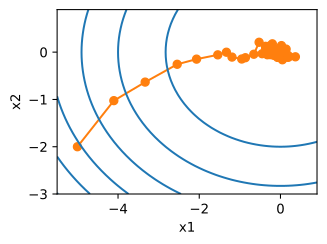
epoch 50, x1: -0.141533, x2: -0.069805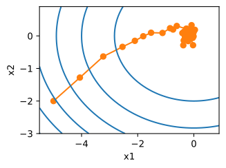
The trajectory is far noisier than the gradient-descent trace in Section 9.2, and, more troubling, it does not settle: run it for more steps and the quality stops improving (we encourage you to check). The reason is visible in the update rule. Near the minimum the true gradient vanishes, but the noise does not, so each step still moves the parameters by \(\eta\) times pure noise. With a constant learning rate the iterates end up executing a random walk around the optimum instead of converging to it. Shrinking \(\eta\) tames the walk but slows the approach; the way out of this bind is to change \(\eta\) during optimization, which is why the step function above threads through a learning rate function lr, dormant so far.
9.3.2 Dynamic Learning Rate
How close does that random walk get? For a quadratic bowl the answer is sharp enough to guide practice. Model one coordinate of the update as \(x_{t+1} = x_t - \eta\, (\lambda x_t + \xi_t)\), with curvature \(\lambda\) and zero-mean noise \(\xi_t\) of variance \(\sigma^2\). Far from the optimum the contraction term dominates and SGD makes gradient-descent-like progress. Close to it, contraction and noise injection balance at
\[\mathbb{E}\big[x_\infty^2\big] \approx \frac{\eta\, \sigma^2}{2\lambda}. \tag{9.3.5}\]
The iterates fluctuate within a noise ball whose squared radius grows linearly with the learning rate. Section 2.1 first introduced this phenomenon. Section 26.1.5 supplies the derivation and compares GD with SGD on the same quadratic objective. Equation Equation 9.3.5 says exactly what the demo showed: a constant \(\eta\) stalls at a noise floor proportional to \(\eta\). Halving \(\eta\) halves the floor — and also halves the speed of the initial approach. A time-dependent learning rate \(\eta(t)\) resolves this tradeoff: large early steps make rapid progress, while smaller later steps reduce the noise floor.
Choosing how fast \(\eta(t)\) decays becomes the new problem. Too fast, and optimization stops prematurely; too slow, and we waste time bouncing in the ball. A few basic strategies (more refined ones follow in Section 9.8):
\[ \begin{aligned} \eta(t) & = \eta_i \textrm{ if } t_i \leq t \leq t_{i+1} && \textrm{piecewise constant} \\ \eta(t) & = \eta_0 \cdot e^{-\lambda t} && \textrm{exponential decay} \\ \eta(t) & = \eta_0 \cdot (\beta t + 1)^{-\alpha} && \textrm{polynomial decay} \end{aligned} \tag{9.3.6}\]
In the piecewise constant scenario we drop the learning rate whenever progress stalls, lowering the noise floor after the iterates reach it. Exponential decay is more aggressive. Polynomial decay with \(\alpha = 0.5\) is a standard well-behaved choice for convex problems. The next experiment shows exponential decay in practice.
def exponential_lr():
    # Global variable that is defined outside this function and updated inside
    global t
    t += 1
    return math.exp(-0.1 * t)

t = 1
lr = exponential_lr
d2l.show_trace_2d(f, d2l.train_2d(sgd, steps=1000, f_grad=f_grad))epoch 1000, x1: -0.769816, x2: -0.084568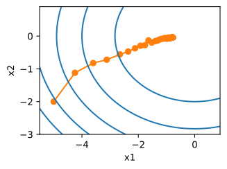
epoch 1000, x1: -0.810909, x2: -0.028332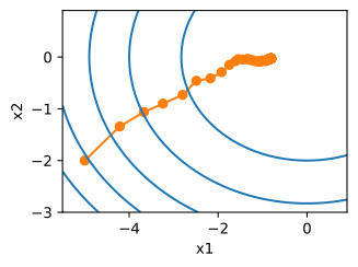
The parameter variance is substantially smaller, but the iterates never reach the optimum \(\mathbf{x} = (0, 0)\), even after 1000 steps. The schedule quenches the noise too eagerly: its total budget \(\sum_t \eta(t)\) is finite, so the iterate can only ever travel a bounded distance from where it started. It stops not because it has arrived but because it has run out of learning rate. Polynomial decay with \(\alpha = 0.5\) avoids that trap, and convergence improves after only 50 steps.
def polynomial_lr():
    # Global variable that is defined outside this function and updated inside
    global t
    t += 1
    return (1 + 0.1 * t) ** (-0.5)

t = 1
lr = polynomial_lr
d2l.show_trace_2d(f, d2l.train_2d(sgd, steps=50, f_grad=f_grad))epoch 50, x1: -0.020206, x2: -0.012148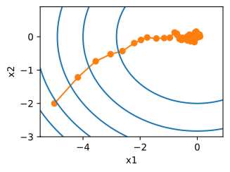
epoch 50, x1: 0.037837, x2: 0.002780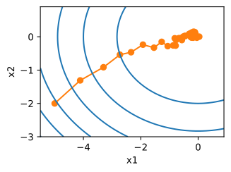
The two experiments are instances of a classical theorem, due to the paper that founded stochastic approximation. Robbins and Monro (1951) showed that convergence requires exactly the two properties the demos probe: the learning rates must sum to infinity, \(\sum_t \eta(t) = \infty\), so the iterate can travel arbitrarily far (the condition exponential decay just violated), while their squares must remain controlled, \(\sum_t \eta(t)^2 < \infty\), so the injected noise is eventually quenched. Polynomial decay with \(\alpha \in (1/2, 1]\) satisfies both; our \(\alpha = 1/2\) sits at the edge of the window, where running for a fixed budget of \(T\) steps with averaged iterates gives the classical \(\mathcal{O}(1/\sqrt{T})\) guarantee for convex objectives. We state these results rather than prove them: the convex rates, and the traps hidden in their constants, are worked out in Section 26.1.5. None of the noise-ball reasoning needs convexity, either — for smooth nonconvex objectives SGD still drives the expected gradient norm to zero at a noise-controlled rate, the theorem of Ghadimi and Lan (2013) proved in Section 26.2.1.
9.3.3 Gradient Variance and Batch Size
So far the noise was ours: we chose \(\sigma = 1\). In real training the noise comes from which examples land in the minibatch, and there we hold a dial — the batch size \(b\). A minibatch gradient averages \(b\) independent draws, so its variance is \(1/b\) times the single-example variance (Section 26.1.5 states and proves this precisely). We test the \(1/b\) prediction on a real network: a small two-layer MLP on the airfoil-noise regression dataset that serves as this chapter’s workhorse from Section 9.4 on. We freeze the parameters at a random initialization, take the full-dataset gradient as ground truth, and measure the mean squared deviation of minibatch gradients from it, for batch sizes spanning nearly three orders of magnitude — sampling with replacement, matching the theory.
data_iter, feature_dim = d2l.get_data_ch11(batch_size=10)
X = torch.cat([Xb for Xb, yb in data_iter])
y = torch.cat([yb for Xb, yb in data_iter])

torch.manual_seed(1)
W1, b1 = torch.randn(feature_dim, 64) * 0.1, torch.zeros(64)
W2, b2 = torch.randn(64, 1) * 0.1, torch.zeros(1)
params = [W1, b1, W2, b2]
for p in params:
    p.requires_grad_(True)

def batch_grad(idx):  # Flattened loss gradient on the minibatch X[idx]
    h = torch.relu(X[idx] @ W1 + b1)
    loss = ((h @ W2 + b2).squeeze() - y[idx]).pow(2).mean() / 2
    return torch.cat([g.reshape(-1) for g in torch.autograd.grad(loss, params)])

g_full = batch_grad(torch.arange(len(y)))
batch_sizes = [1, 8, 64, 512]
var = []
for b in batch_sizes:
    idx = torch.randint(0, len(y), (200, b))
    var.append(torch.stack([((batch_grad(i) - g_full) ** 2).sum()
                            for i in idx]).mean().item())
d2l.plot(batch_sizes, [var, [var[0] / b for b in batch_sizes]],
         'batch size', 'gradient variance', xscale='log', yscale='log',
         legend=['measured', '1/b'])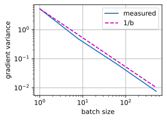
data_iter, feature_dim = d2l.get_data_ch11(batch_size=10)
X = jnp.concatenate([jnp.asarray(Xb) for Xb, yb in data_iter])
y = jnp.concatenate([jnp.asarray(yb) for Xb, yb in data_iter])

k1, k2 = jax.random.split(jax.random.PRNGKey(1))
params = dict(W1=0.1 * jax.random.normal(k1, (feature_dim, 64)),
              b1=jnp.zeros(64),
              W2=0.1 * jax.random.normal(k2, (64, 1)), b2=jnp.zeros(1))

def batch_loss(params, idx):
    h = jax.nn.relu(X[idx] @ params['W1'] + params['b1'])
    return jnp.mean(((h @ params['W2'] + params['b2']).squeeze()
                     - y[idx]) ** 2) / 2

def batch_grad(idx):  # Flattened loss gradient on the minibatch X[idx]
    grads = jax.grad(batch_loss)(params, idx)
    return jnp.concatenate([g.reshape(-1) for g in jax.tree.leaves(grads)])

g_full = batch_grad(jnp.arange(len(y)))
batch_sizes = [1, 8, 64, 512]
var, key = [], jax.random.PRNGKey(0)
for b in batch_sizes:
    key, subkey = jax.random.split(key)
    idx = jax.random.randint(subkey, (200, b), 0, len(y))
    err = jax.vmap(lambda i: ((batch_grad(i) - g_full) ** 2).sum())(idx)
    var.append(float(err.mean()))
d2l.plot(batch_sizes, [var, [var[0] / b for b in batch_sizes]],
         'batch size', 'gradient variance', xscale='log', yscale='log',
         legend=['measured', '1/b'])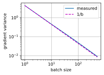
The measured points fall on the \(1/b\) reference line across the whole range: a factor of 500 in batch size reduces the variance by the same factor. Note what the log scale conceals. Variance falling like \(1/b\) means noise amplitude falls like \(1/\sqrt{b}\), so spending \(100\times\) more compute per step reduces the noise amplitude by only a factor of \(10\). Batch size is thus a genuine second dial next to the learning rate, but one with diminishing returns. Section 9.4 takes up how to spend a compute budget between the two, and how batching interacts with the hardware that made it cheap; Section 9.10 asks when the \(1/b\) variance reduction stops improving data efficiency at the scale of modern language models.
One loose end. Our theory and the measurement above both sampled indices with replacement: each draw is independent, which is what makes the analysis clean. Practice does something else. Drawing \(n\) times with replacement touches only a fraction \(1 - (1-1/n)^n \approx 1 - e^{-1} \approx 0.63\) of the dataset per pass while picking other examples twice or more — lower data efficiency and higher variance than shuffling the dataset and traversing it exactly once per epoch. So that is what every training loop in this book does, reshuffling before each epoch. The cost is theoretical: within an epoch, successive gradients are no longer independent, and the clean proofs no longer apply verbatim. The gap is real but benign in practice, and the exercises take it up.
9.3.4 Summary
SGD trades exactness for speed: an unbiased \(\mathcal{O}(1)\)-per-step gradient estimate in place of an \(\mathcal{O}(n)\) exact one. This introduces variance, and this section met both of the dials that control it. A constant learning rate leaves the iterates rattling in a noise ball of squared radius proportional to \(\eta\); decaying learning rates converge, provided the decay permits unbounded cumulative movement while making the accumulated noise finite. Batch size is the other dial: minibatch gradient variance falls like \(1/b\), measured on a real network over a factor of 500 in batch size, though at a linear cost in compute per step. The proofs owed here live in Section 26.1.5 and Section 26.2.1: the convex rates and the nonconvex Ghadimi–Lan theorem.
9.3.5 Exercises
- [code] Schedules on the noisy quadratic.
sgdwithconstant_lr,exponential_lr, andpolynomial_lrruns a constant learning rate and two of the schedules in Equation 9.3.6 on \(f(x_1, x_2) = x_1^2 + 2x_2^2\).- Run all three for 1,000 steps from the starting point of
d2l.train_2d. Plot the distance \(\|\mathbf{x}_t\|\) to the optimum, averaged over 20 runs, against \(t\) on a logarithmic scale. Which schedule is closest after 50 steps, and which after 1,000? - Write \(B = \sum_t \eta(t)\) for the total budget, where \(\eta(t)\) is the step size
eta * lr()thatsgdapplies at step \(t\). Show that without noise \(x_1\) shrinks over the run by a factor of about \(e^{-2B}\). Compute \(B\) forexponential_lrand compare the predicted final \(x_1\) with the run. Then choose a decay constant whose predicted final \(|x_1|\) is below \(0.01\), and compare the final distance of this run with that ofpolynomial_lr, again averaged over 20 runs.
- Run all three for 1,000 steps from the starting point of
- Piecewise constant decay. Piecewise constant decay with finitely many drops is not covered by the Robbins–Monro conditions. Which of the two conditions does it violate, and why is it nonetheless a sensible choice when the number of steps is fixed in advance?
- Noise as a random dataset. The simulation in
sgdadds Gaussian noise to the gradient of \(f(x_1, x_2) = x_1^2 + 2x_2^2\). Prove that this is equivalent to stochastic gradient descent on the per-example losses \(f(\mathbf{x}, \mathbf{w}) = (x_1 - w_1)^2 + 2(x_2 - w_2)^2\) with \(\mathbf{w}\) drawn from a normal distribution, and state the covariance of \(\mathbf{w}\) that reproduces unit-variance noise in both gradient coordinates. - [code] Reshuffling versus replacement. ● Draw a dataset of \(n = 100\) vectors \(\mathbf{w}_i\) from the distribution of the previous problem and run SGD on the resulting finite sum for 20 epochs, once sampling \(i\) with replacement and once reshuffling the dataset before each epoch. Record the distance to the finite-sum minimizer after each epoch, averaged over 20 seeds, at the constant learning rates \(\eta = 0.1\) and \(\eta = 0.01\). At which learning rate does reshuffling make the larger difference, and why?
- [code] Anisotropic noise ball. ● The estimate Equation 9.3.5 applies to each coordinate separately, with curvatures \(\lambda_1 = 2\) and \(\lambda_2 = 4\) for the quadratic used in
sgd.- Run
sgdwithconstant_lrat \(\eta = 0.1\) for 10,000 steps and estimate the stationary variance of \(x_1\) and of \(x_2\) from the last 5,000 iterates. Compare both with Equation 9.3.5. Then derive the exact stationary variance of the recursion \(x_{t+1} = x_t - \eta\, (\lambda x_t + \xi_t)\) and explain for which coordinate the approximation is worse. - Give each coordinate its own learning rate \(\eta_i = \eta / \lambda_i\). Derive how the contraction factor \(1 - \eta_i \lambda_i\) and the noise floor \(\eta_i \sigma^2 / (2\lambda_i)\) change, and explain why this choice needs information that a gradient alone does not supply.
- Implement the per-coordinate rates in
sgdand verify both predictions of the previous item numerically.
- Run
- [code] Gradient variance after training. ● The measurement in Section 9.3.3 froze the two-layer network at a random initialization. Train it on the airfoil data for ten epochs of minibatch SGD with batch size 10 and learning rate 0.05, reshuffling the examples before each epoch. At initialization and again after training, recompute
g_fullwithbatch_gradand compute the single-example gradient variance exactly by averaging the squared deviation over all 1,500 examples. Split this variance into the contributions ofW1,b1,W2, andb2, and explain the changes in theb2andW1contributions from the form of the per-example gradient of the squared loss.