from d2l import torch as d2l
import torch
from torch import nn6.5 Pooling
Many image tasks require a global prediction, such as whether an image contains a cat. The final representation must therefore combine information from the entire input. Convolutional networks commonly build this representation by progressively reducing spatial resolution while increasing the receptive field of each hidden unit. Deeper hidden units have larger receptive fields relative to the input. Reducing spatial resolution accelerates this growth because subsequent kernels cover a larger effective area.
For lower-level features such as edges, we also want small translations of the input to produce modest changes in the representation. For instance, if we take the image X with a sharp delineation between black and white and shift the whole image by one pixel to the right, i.e., Z[i, j] = X[i, j - 1], then the edge in the new output shifts by one pixel and sampled values may change. Such shifts occur whenever an object or camera moves slightly.
This section introduces pooling layers, which summarize local windows to reduce spatial resolution and sensitivity to small translations.
from d2l import tensorflow as d2l
import tensorflow as tf
from d2l import jax as d2l
from flax import nnx
import jax
from jax import numpy as jnpfrom d2l import mxnet as d2l
from mxnet import np, npx
from mxnet.gluon import nn
npx.set_np()6.5.1 Maximum Pooling and Average Pooling
Like convolutional layers, pooling operators consist of a fixed-shape window that is slid over all regions in the input according to its stride, computing a single output for each location traversed by the fixed-shape window (sometimes known as the pooling window). However, unlike the cross-correlation computation of the inputs and kernels in the convolutional layer, the pooling layer contains no parameters (there is no kernel). Instead, pooling operators are deterministic, typically calculating either the maximum or the average value of the elements in the pooling window. These operations are called maximum pooling (max-pooling for short) and average pooling, respectively.
Average pooling dates to the earliest CNNs and resembles image downsampling. Instead of retaining every second or third pixel, it averages adjacent pixels, combining their information and reducing high-frequency variation. Max-pooling was introduced in Riesenhuber and Poggio (1999) in the context of cognitive neuroscience to describe how information might be aggregated hierarchically for the purpose of object recognition; there already was an earlier version in speech recognition (Yamaguchi et al. 1990). Historically, max-pooling was often preferred inside convolutional bodies, while average pooling became the standard choice for global classifier heads. Neither dominates in every setting.
In both cases, as with the cross-correlation operator, we can think of the pooling window as starting from the upper-left of the input tensor and sliding across it from left to right and top to bottom. At each location that the pooling window hits, it computes the maximum or average value of the input subtensor in the window, depending on whether max or average pooling is employed.
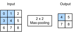
The output tensor in Figure 6.5.1 has a height of 2 and a width of 2. The four elements are derived from the maximum value in each pooling window:
\[ \begin{aligned} \max(0, 1, 3, 4) &= 4,\\ \max(1, 2, 4, 5) &= 5,\\ \max(3, 4, 6, 7) &= 7,\\ \max(4, 5, 7, 8) &= 8. \end{aligned} \]
More generally, we can define a \(p \times q\) pooling layer by aggregating over a region of that size. Returning to the problem of edge detection, we use the output of the convolutional layer as input for \(2\times 2\) max-pooling. Denote the edge-detector output by X and the pooling output by Y. If a single response of value 1 moves anywhere within the same \(2\times2\) pooling window while the other responses remain no larger, then Y[i, j] remains 1. Thus max-pooling can make a representation insensitive to some small movements that stay within a window. Crossing a window boundary can still change the pooled output abruptly, so this is local tolerance rather than exact translation invariance.
In the code below, we implement the forward propagation of the pooling layer in the pool2d function. This function is similar to the corr2d function in Section 6.2. No kernel is needed: the output is the maximum or the average of each region in the input.
def pool2d(X, pool_size, mode='max'):
    p_h, p_w = pool_size
    Y = d2l.zeros((X.shape[0] - p_h + 1, X.shape[1] - p_w + 1))
    for i in range(Y.shape[0]):
        for j in range(Y.shape[1]):
            if mode == 'max':
                Y[i, j] = X[i: i + p_h, j: j + p_w].max()
            elif mode == 'avg':
                Y[i, j] = X[i: i + p_h, j: j + p_w].mean()
    return Y
def pool2d(X, pool_size, mode='max'):
p_h, p_w = pool_size
Y = tf.Variable(tf.zeros((X.shape[0] - p_h + 1, X.shape[1] - p_w +1)))
for i in range(Y.shape[0]):
for j in range(Y.shape[1]):
if mode == 'max':
Y[i, j].assign(tf.reduce_max(X[i: i + p_h, j: j + p_w]))
elif mode =='avg':
Y[i, j].assign(tf.reduce_mean(X[i: i + p_h, j: j + p_w]))
return Ydef pool2d(X, pool_size, mode='max'):
p_h, p_w = pool_size
Y = jnp.zeros((X.shape[0] - p_h + 1, X.shape[1] - p_w + 1))
for i in range(Y.shape[0]):
for j in range(Y.shape[1]):
if mode == 'max':
Y = Y.at[i, j].set(X[i: i + p_h, j: j + p_w].max())
elif mode == 'avg':
Y = Y.at[i, j].set(X[i: i + p_h, j: j + p_w].mean())
return Ydef pool2d(X, pool_size, mode='max'):
p_h, p_w = pool_size
Y = d2l.zeros((X.shape[0] - p_h + 1, X.shape[1] - p_w + 1))
for i in range(Y.shape[0]):
for j in range(Y.shape[1]):
if mode == 'max':
Y[i, j] = X[i: i + p_h, j: j + p_w].max()
elif mode == 'avg':
Y[i, j] = X[i: i + p_h, j: j + p_w].mean()
return YWe can construct the input tensor X in Figure 6.5.1 to validate the output of the two-dimensional max-pooling layer.
X = d2l.tensor([[0.0, 1.0, 2.0], [3.0, 4.0, 5.0], [6.0, 7.0, 8.0]])
pool2d(X, (2, 2))tensor([[4., 5.],
[7., 8.]])<tf.Variable 'Variable:0' shape=(2, 2) dtype=float32, numpy=
array([[4., 5.],
[7., 8.]], dtype=float32)>Array([[4., 5.],
[7., 8.]], dtype=float32)array([[4., 5.],
[7., 8.]])We can likewise evaluate average pooling.
pool2d(X, (2, 2), 'avg')tensor([[2., 3.],
[5., 6.]])<tf.Variable 'Variable:0' shape=(2, 2) dtype=float32, numpy=
array([[2., 3.],
[5., 6.]], dtype=float32)>Array([[2., 3.],
[5., 6.]], dtype=float32)array([[2., 3.],
[5., 6.]])6.5.2 Padding and Stride
As with convolutional layers, pooling layers change the output shape. And as before, we can adjust the operation to achieve a desired output shape by padding the input and adjusting the stride. We can demonstrate the use of padding and strides in pooling layers via the built-in two-dimensional max-pooling layer from the deep learning framework. We first construct an input tensor X whose shape has four dimensions, where the number of examples (batch size) and number of channels are both 1.
Unlike the other frameworks, TensorFlow prefers and is optimized for channels-last input.
X = d2l.reshape(d2l.arange(16, dtype=d2l.float32), (1, 1, 4, 4))
X
tensor([[[[ 0., 1., 2., 3.],
[ 4., 5., 6., 7.],
[ 8., 9., 10., 11.],
[12., 13., 14., 15.]]]])X = d2l.reshape(d2l.arange(16, dtype=d2l.float32), (1, 4, 4, 1))
X<tf.Tensor: shape=(1, 4, 4, 1), dtype=float32, numpy=
array([[[[ 0.],
[ 1.],
[ 2.],
[ 3.]],
[[ 4.],
[ 5.],
[ 6.],
[ 7.]],
[[ 8.],
[ 9.],
[10.],
[11.]],
[[12.],
[13.],
[14.],
[15.]]]], dtype=float32)>X = d2l.reshape(d2l.arange(16, dtype=d2l.float32), (1, 4, 4, 1))
XArray([[[[ 0.],
[ 1.],
[ 2.],
[ 3.]],
[[ 4.],
[ 5.],
[ 6.],
[ 7.]],
[[ 8.],
[ 9.],
[10.],
[11.]],
[[12.],
[13.],
[14.],
[15.]]]], dtype=float32)X = d2l.reshape(d2l.arange(16, dtype=d2l.float32), (1, 1, 4, 4))
Xarray([[[[ 0., 1., 2., 3.],
[ 4., 5., 6., 7.],
[ 8., 9., 10., 11.],
[12., 13., 14., 15.]]]])Since pooling aggregates information from an area, deep learning frameworks default to matching pooling window sizes and stride. For instance, if we use a pooling window of shape (3, 3) we get a stride shape of (3, 3) by default.
pool2d = nn.MaxPool2d(3)
# Pooling has no model parameters, hence it needs no initialization
pool2d(X)tensor([[[[10.]]]])pool2d = tf.keras.layers.MaxPool2D(pool_size=[3, 3])
# Pooling has no model parameters, hence it needs no initialization
pool2d(X)<tf.Tensor: shape=(1, 1, 1, 1), dtype=float32, numpy=array([[[[10.]]]], dtype=float32)># Pooling has no model parameters, hence it needs no initialization
nnx.max_pool(X, window_shape=(3, 3), strides=(3, 3))Array([[[[10.]]]], dtype=float32)pool2d = nn.MaxPool2D(3)
# Pooling has no model parameters, hence it needs no initialization
pool2d(X)array([[[[10.]]]])The stride and padding can be specified explicitly to override the framework defaults.
pool2d = nn.MaxPool2d(3, padding=1, stride=2)
pool2d(X)
tensor([[[[ 5., 7.],
[13., 15.]]]])paddings = tf.constant([[0, 0], [1,0], [1,0], [0,0]])
X_padded = tf.pad(X, paddings, "CONSTANT")
pool2d = tf.keras.layers.MaxPool2D(pool_size=[3, 3], padding='valid',
strides=2)
pool2d(X_padded)<tf.Tensor: shape=(1, 2, 2, 1), dtype=float32, numpy=
array([[[[ 5.],
[ 7.]],
[[13.],
[15.]]]], dtype=float32)>X_padded = jnp.pad(X, ((0, 0), (1, 0), (1, 0), (0, 0)), mode='constant')
nnx.max_pool(X_padded, window_shape=(3, 3), padding='VALID', strides=(2, 2))Array([[[[ 5.],
[ 7.]],
[[13.],
[15.]]]], dtype=float32)pool2d = nn.MaxPool2D(3, padding=1, strides=2)
pool2d(X)array([[[[ 5., 7.],
[13., 15.]]]])Pooling windows can also have different heights and widths.
pool2d = nn.MaxPool2d((2, 3), stride=(2, 3), padding=(0, 1))
pool2d(X)
tensor([[[[ 5., 7.],
[13., 15.]]]])paddings = tf.constant([[0, 0], [0, 0], [1, 1], [0, 0]])
X_padded = tf.pad(X, paddings, "CONSTANT")
pool2d = tf.keras.layers.MaxPool2D(pool_size=[2, 3], padding='valid',
strides=(2, 3))
pool2d(X_padded)<tf.Tensor: shape=(1, 2, 2, 1), dtype=float32, numpy=
array([[[[ 5.],
[ 7.]],
[[13.],
[15.]]]], dtype=float32)>
X_padded = jnp.pad(X, ((0, 0), (0, 0), (1, 1), (0, 0)), mode='constant')
nnx.max_pool(X_padded, window_shape=(2, 3), strides=(2, 3), padding='VALID')
Array([[[[ 5.],
[ 7.]],
[[13.],
[15.]]]], dtype=float32)pool2d = nn.MaxPool2D((2, 3), padding=(0, 1), strides=(2, 3))
pool2d(X)array([[[[ 5., 7.],
[13., 15.]]]])6.5.3 Multiple Channels
When processing multi-channel input data, the pooling layer pools each input channel separately, rather than summing the inputs up over channels as in a convolutional layer. This means that the number of output channels for the pooling layer is the same as the number of input channels. Below, we will concatenate tensors X and X + 1 on the channel dimension to construct an input with two channels.
TensorFlow’s channels-last layout requires concatenation along the final dimension.
X = d2l.concat((X, X + 1), 1)
X
tensor([[[[ 0., 1., 2., 3.],
[ 4., 5., 6., 7.],
[ 8., 9., 10., 11.],
[12., 13., 14., 15.]],
[[ 1., 2., 3., 4.],
[ 5., 6., 7., 8.],
[ 9., 10., 11., 12.],
[13., 14., 15., 16.]]]])# Concatenate along `dim=3` due to channels-last syntax
X = d2l.concat([X, X + 1], 3)
X<tf.Tensor: shape=(1, 4, 4, 2), dtype=float32, numpy=
array([[[[ 0., 1.],
[ 1., 2.],
[ 2., 3.],
[ 3., 4.]],
[[ 4., 5.],
[ 5., 6.],
[ 6., 7.],
[ 7., 8.]],
[[ 8., 9.],
[ 9., 10.],
[10., 11.],
[11., 12.]],
[[12., 13.],
[13., 14.],
[14., 15.],
[15., 16.]]]], dtype=float32)># Concatenate along `dim=3` due to channels-last syntax
X = d2l.concat([X, X + 1], 3)
XArray([[[[ 0., 1.],
[ 1., 2.],
[ 2., 3.],
[ 3., 4.]],
[[ 4., 5.],
[ 5., 6.],
[ 6., 7.],
[ 7., 8.]],
[[ 8., 9.],
[ 9., 10.],
[10., 11.],
[11., 12.]],
[[12., 13.],
[13., 14.],
[14., 15.],
[15., 16.]]]], dtype=float32)X = d2l.concat((X, X + 1), 1)
Xarray([[[[ 0., 1., 2., 3.],
[ 4., 5., 6., 7.],
[ 8., 9., 10., 11.],
[12., 13., 14., 15.]],
[[ 1., 2., 3., 4.],
[ 5., 6., 7., 8.],
[ 9., 10., 11., 12.],
[13., 14., 15., 16.]]]])The output still has two channels after pooling.
pool2d = nn.MaxPool2d(3, padding=1, stride=2)
pool2d(X)
tensor([[[[ 5., 7.],
[13., 15.]],
[[ 6., 8.],
[14., 16.]]]])paddings = tf.constant([[0, 0], [1,0], [1,0], [0,0]])
X_padded = tf.pad(X, paddings, "CONSTANT")
pool2d = tf.keras.layers.MaxPool2D(pool_size=[3, 3], padding='valid',
strides=2)
pool2d(X_padded)<tf.Tensor: shape=(1, 2, 2, 2), dtype=float32, numpy=
array([[[[ 5., 6.],
[ 7., 8.]],
[[13., 14.],
[15., 16.]]]], dtype=float32)>X_padded = jnp.pad(X, ((0, 0), (1, 0), (1, 0), (0, 0)), mode='constant')
nnx.max_pool(X_padded, window_shape=(3, 3), padding='VALID', strides=(2, 2))Array([[[[ 5., 6.],
[ 7., 8.]],
[[13., 14.],
[15., 16.]]]], dtype=float32)pool2d = nn.MaxPool2D(3, padding=1, strides=2)
pool2d(X)array([[[[ 5., 7.],
[13., 15.]],
[[ 6., 8.],
[14., 16.]]]])TensorFlow stores these tensors in NHWC order, whereas the MXNet and PyTorch tabs use NCHW order. Transposing the TensorFlow result from NHWC to NCHW gives the same values; only the channel axis is displayed in a different position.
6.5.4 Summary
Pooling is a simple operation: it replaces each window of values with a single summary, the maximum or the mean. The stride and padding semantics of convolutions carry over unchanged, and pooling applies to each channel separately, so the number of channels is preserved. There are no parameters to learn. A \(2 \times 2\) window with stride 2, which quarters the number of spatial locations, is the classical local configuration; global average pooling is now the common classification head.
Modern convolutional networks often reduce resolution with strided convolutions: a convolution with stride 2 halves the resolution while learning its aggregation weights instead of fixing them to a maximum or mean. ResNet (Section 7.4) uses this pattern within its stages. Pooling remains common in two roles. Global average pooling, introduced with the network-in-network architecture (Section 7.2.2) (Lin et al. 2013), averages each channel over all spatial positions and turns the final feature map into one value per channel. It often replaces the large fully connected classifier stacks of early CNNs. Max-pooling persists in some network stems and in detection models that combine feature maps across scales.
One caveat applies to every stride-2 downsampler, pooled or convolutional: subsampling a signal without first removing its high spatial frequencies can alias, so that shifting the input by a single pixel changes the output noticeably; applying a small low-pass (blur) filter before subsampling can make the result substantially more shift-consistent, though not exactly invariant (Zhang 2019). Beyond these mainstays there are randomized variants such as stochastic pooling (Zeiler and Fergus 2013) and fractional max-pooling (Graham 2014), and the attention mechanisms of Chapter 10 aggregate by learned alignment between a query and representation vectors rather than by spatial location.
6.5.5 Exercises
[code] Average pooling as convolution. Express \(k_\textrm{h} \times k_\textrm{w}\) average pooling with stride \((s_\textrm{h}, s_\textrm{w})\) as a convolution. Give the kernel, and state how the convolution must be structured across channels so that each channel is pooled separately, as pooling layers do. On the input
Xof Figure 6.5.1, verify that your convolution reproducespool2d(X, (2, 2), 'avg'), wherepool2dis the function defined at the start of this section.Max-pooling via ReLU. ●
- Prove that max-pooling cannot be implemented by a convolution alone.
- Express \(\max(a, b)\) using only affine operations and \(\textrm{ReLU}(x) = \max(0, x)\).
- Use this to implement max-pooling as a stack of convolutions and ReLU layers.
- Count the channels per layer and the ReLU layers that your construction uses for a \(2 \times 2\) window and for a \(3 \times 3\) window. How does the number of ReLU layers grow with the number of entries in the window?
Cost of pooling. An input of shape \(c \times n_\textrm{h} \times n_\textrm{w}\) is pooled with a \(k_\textrm{h} \times k_\textrm{w}\) window, total padding \((p_\textrm{h}, p_\textrm{w})\), and stride \((s_\textrm{h}, s_\textrm{w})\).
- Count the comparisons that max-pooling performs and the additions that average pooling performs. Take the output shape from Equation 6.3.4 with dilation 1.
- Compare these counts with the number of multiply-adds of a convolution with the same window, padding, and stride and with \(c\) input and \(c\) output channels. By roughly which factor is pooling cheaper?
[code] Max versus average pooling. Construct two synthetic \(4 \times 4\) patches with the same mean: one with a single high-value outlier on a uniform background, and one with a smooth gradient. Apply \(2 \times 2\) max-pooling and average pooling with stride 2 to both and report all four outputs. Using these numbers, describe one scenario in which max-pooling is preferable and one in which average pooling is preferable.
Pooling alternatives.
- Do we need a separate minimum-pooling layer, or can it be expressed through an operation already in this section?
- Softmax pooling with temperature \(\tau > 0\) replaces the window entries \(x_1, \ldots, x_m\) by their softmax-weighted average \[\sum_{i=1}^m x_i \frac{\exp(x_i / \tau)}{\sum_{j=1}^m \exp(x_j / \tau)}. \tag{6.5.1}\] Find its limits as \(\tau \to 0\) and as \(\tau \to \infty\). Give one cost that softmax pooling adds relative to max-pooling.
Aliasing and blur-pool. Naive stride-2 downsampling keeps every second entry of its input. Measure frequency in cycles per input sample, so that the one-dimensional signals \((1, 0, 1, 0, 1, 0)\) and \((0, 1, 0, 1, 0, 1)\) both have frequency \(\tfrac{1}{2}\).
- Apply naive stride-2 downsampling to both signals, which differ by a shift of one position, and compare the two outputs. Why is this behavior called aliasing?
- Which input frequencies can a stride-2 subsampler represent faithfully?
- Blur-pool (Zhang 2019) counteracts aliasing by applying a small averaging filter before subsampling. Work out what blur-pool with a two-tap box filter \((\tfrac{1}{2}, \tfrac{1}{2})\) computes on the two signals above. Which pooling operation from this section does it coincide with?
[code] Backward pass of max-pooling. Derive the gradient of two-dimensional max-pooling with respect to its input, for a \(k_\textrm{h} \times k_\textrm{w}\) window and stride equal to the window size, and implement it without automatic differentiation. Verify against the gradient that automatic differentiation computes through the built-in max-pooling operation of this section on a small random tensor, to a relative error below \(10^{-4}\).
Adapted from Stanford CS231n, Assignment 2, ConvolutionalNetworks, naive max-pooling backward pass.