%matplotlib inline
from d2l import torch as d2l
import torch
from torch import nn11.5 Vision Transformer
The transformer models considered so far operate on text, but their blocks process vectors without assuming that they represent words. This section applies the same blocks to vectors obtained from image patches.
Convolutional networks encode locality and translation equivariance (Section 6.1), whereas a plain transformer block does not. Early attention-based vision models retained local structure: Ramachandran et al. (2019) used local self-attention, and Cordonnier et al. (2020) analyzed conditions under which self-attention can express convolutional operations. The vision transformer (ViT) of Dosovitskiy et al. (2021) divides an image into \(16 \times 16\) patches, embeds each patch as a token, and applies an unmodified transformer encoder to the resulting sequence. In the ViT paper’s JFT-300M pretraining and downstream fine-tuning protocol, the largest reported ViT variants exceeded the cited convolutional baselines on several classification benchmarks. That comparison changes data, model size, compute, augmentation, and pretraining together; it does not isolate data scale as the cause.
We build this model and train it on Fashion-MNIST, then compare it with a CNN at the same parameter count and training budget. The CNN performs better in this protocol. Its architectural priors are one plausible contributor, but the comparison does not isolate their causal effect. We also inspect whether the learned position embeddings reflect the \(6 \times 6\) patch grid.
%matplotlib inline
from d2l import jax as d2l
from flax import nnx
import jax
from jax import numpy as jnp
11.5.1 Patches as Tokens
Figure 11.5.1 depicts the architecture. It consists of a stem that patchifies images, a body of transformer blocks, and a head that turns one token’s final representation into a class label.
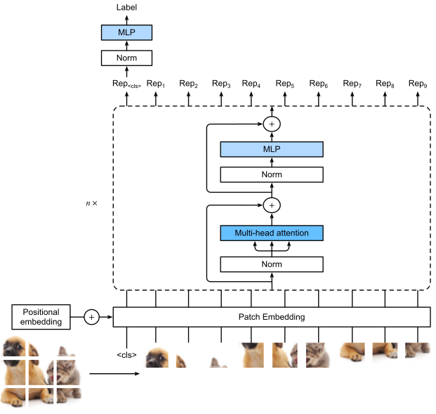
Consider an input image with height \(h\), width \(w\), and \(c\) channels. With patch height and width both set to \(p\), the image is split into a sequence of \(m = hw/p^2\) patches, each flattened to a vector of length \(cp^2\). A special “<cls>” (class) token and the \(m\) flattened patches are linearly projected into \(m + 1\) vectors and summed with learnable positional embeddings. From here on the model is the encoder wiring of Section 11.4: a stack of transformer blocks with no causal mask, every token attending to every other, mapping \(m + 1\) input vectors to \(m + 1\) output representations of the same dimension. Since the “<cls>” token attends to all the image patches, its representation at the output of the stack summarizes the whole image and is the one the classification head reads.
Splitting an image into patches and linearly projecting the flattened patches sounds like two operations, but they combine into one: a convolution whose kernel size and stride both equal the patch size. Each output position of such a convolution sees exactly one patch and computes exactly its linear projection.
class PatchEmbedding(nn.Module):
    """Image-to-sequence stem of the vision transformer."""
    def __init__(self, img_size=96, patch_size=16, num_hiddens=512):
        super().__init__()
        def _make_tuple(x):
            if not isinstance(x, (list, tuple)):
                return (x, x)
            return x
        img_size, patch_size = _make_tuple(img_size), _make_tuple(patch_size)
        # A partial trailing patch would silently shrink the token grid
        assert img_size[0] % patch_size[0] == 0 and \
            img_size[1] % patch_size[1] == 0, \
            'image size must be divisible by the patch size'
        self.num_patches = (img_size[0] // patch_size[0]) * (
            img_size[1] // patch_size[1])
        self.conv = nn.LazyConv2d(num_hiddens, kernel_size=patch_size,
                                  stride=patch_size)

    def forward(self, X):
        # Output shape: (batch size, no. of patches, no. of channels)
        return self.conv(X).flatten(2).transpose(1, 2)
class PatchEmbedding(nnx.Module):
"""Image-to-sequence stem of the vision transformer."""
def __init__(self, img_size=96, patch_size=16, num_hiddens=512,
num_channels=3, rngs=None):
rngs = nnx.Rngs(0) if rngs is None else rngs
def _make_tuple(x):
if not isinstance(x, (list, tuple)):
return (x, x)
return x
img_size, patch_size = _make_tuple(img_size), _make_tuple(patch_size)
# A partial trailing patch would silently shrink the token grid
assert img_size[0] % patch_size[0] == 0 and \
img_size[1] % patch_size[1] == 0, \
'image size must be divisible by the patch size'
self.num_patches = (img_size[0] // patch_size[0]) * (
img_size[1] // patch_size[1])
self.conv = nnx.Conv(num_channels, num_hiddens, kernel_size=patch_size,
strides=patch_size, padding='VALID', rngs=rngs)
def __call__(self, X):
# Output shape: (batch size, no. of patches, no. of channels)
X = self.conv(X)
return X.reshape((X.shape[0], -1, X.shape[3]))In the following example, taking images with height and width of img_size as inputs, the patch embedding outputs (img_size//patch_size)**2 patches that are linearly projected to vectors of length num_hiddens.
img_size, patch_size, num_hiddens, batch_size = 96, 16, 512, 4
patch_emb = PatchEmbedding(img_size, patch_size, num_hiddens)
X = d2l.zeros(batch_size, 3, img_size, img_size)
d2l.check_shape(patch_emb(X),
                (batch_size, (img_size//patch_size)**2, num_hiddens))
img_size, patch_size, num_hiddens, batch_size = 96, 16, 512, 4
patch_emb = PatchEmbedding(img_size, patch_size, num_hiddens)
X = d2l.zeros((batch_size, img_size, img_size, 3))
d2l.check_shape(patch_emb(X),
(batch_size, (img_size//patch_size)**2, num_hiddens))This patch projection is the interface between the image and the transformer. Subsequent blocks process the patch vectors in the same form as token embeddings.
11.5.2 The Vision Transformer Block
The body of the model is the transformer block of Section 11.1 in its pre-norm configuration: normalization sits on each branch, right before multi-head attention and before the MLP, and the residual stream runs uninterrupted. ViT adopted this arrangement as analyses began to establish its training advantages (Baevski and Auli 2018; Wang et al. 2019; Xiong et al. 2020). Pre-norm subsequently became common in transformer architectures.
Two details are specific to the vision variant. The MLP uses the Gaussian error linear unit (GELU), a smooth relative of ReLU (Hendrycks and Gimpel 2016), and applies dropout after each of its two linear layers. Dropout is retained in the ViT training recipe, unlike in many large language-model recipes. And because every patch is a valid token that may look at every other, the block needs no mask: the valid_lens argument of the d2l.MultiHeadAttention from Section 10.3 stays None throughout this section.
class ViTBlock(nn.Module):
    """Pre-norm transformer block with a GELU MLP."""
    def __init__(self, num_hiddens, mlp_num_hiddens, num_heads, dropout,
                 use_bias=False):
        super().__init__()
        self.ln1 = nn.LayerNorm(num_hiddens)
        self.attention = d2l.MultiHeadAttention(num_hiddens, num_heads,
                                                dropout, use_bias)
        self.ln2 = nn.LayerNorm(num_hiddens)
        self.mlp = nn.Sequential(
            nn.LazyLinear(mlp_num_hiddens), nn.GELU(), nn.Dropout(dropout),
            nn.LazyLinear(num_hiddens), nn.Dropout(dropout))

    def forward(self, X, valid_lens=None):
        X = X + self.attention(*([self.ln1(X)] * 3), valid_lens)
        return X + self.mlp(self.ln2(X))
class ViTBlock(nnx.Module):
"""Pre-norm transformer block with a GELU MLP."""
def __init__(self, num_hiddens, mlp_num_hiddens, num_heads, dropout,
use_bias=False, rngs=None):
rngs = nnx.Rngs(params=0, dropout=1) if rngs is None else rngs
self.ln1 = nnx.LayerNorm(num_hiddens, rngs=rngs)
self.attention = d2l.MultiHeadAttention(
num_hiddens, num_heads, dropout, use_bias, rngs=rngs)
self.ln2 = nnx.LayerNorm(num_hiddens, rngs=rngs)
self.mlp = nnx.Sequential(
nnx.Linear(num_hiddens, mlp_num_hiddens, rngs=rngs), nnx.gelu,
nnx.Dropout(dropout, rngs=rngs),
nnx.Linear(mlp_num_hiddens, num_hiddens, rngs=rngs),
nnx.Dropout(dropout, rngs=rngs))
def __call__(self, X, valid_lens=None):
X_norm = self.ln1(X)
X = X + self.attention(X_norm, X_norm, X_norm, valid_lens)[0]
return X + self.mlp(self.ln2(X))As with every transformer block, the output shape equals the input shape, so the blocks can be stacked directly.
X = d2l.ones((2, 100, 24))
encoder_blk = ViTBlock(24, 48, 8, 0.5)
encoder_blk.eval()
d2l.check_shape(encoder_blk(X), X.shape)
X = d2l.ones((2, 100, 24))
encoder_blk = ViTBlock(24, 48, 8, 0.5)
d2l.check_shape(nnx.view(encoder_blk, deterministic=True)(X), X.shape)11.5.3 The Full Model
Assembling the pieces takes one class. Input images pass through a PatchEmbedding instance; a learnable “<cls>” token embedding, initialized to zeros, is prepended to the resulting sequence. The sum with the positional embeddings goes through dropout, then through num_blks stacked ViTBlock instances, and finally the head projects the “<cls>” token’s representation to the class logits.
The positional embeddings must represent a two-dimensional grid. The sinusoidal and rotary constructions of Section 10.4 encode positions along a line, but a patch has a row and a column, and it is not obvious what a hand-designed two-dimensional code should look like. ViT sidesteps the question: the position embeddings are a freely learnable parameter, initialized to small Gaussian noise as in the original recipe, one vector per sequence position. At initialization, the model therefore does not encode that patch 7 lies directly left of patch 8 and directly above patch 13; the patches enter as an unordered set of vectors. Whatever spatial structure the trained model uses, it must discover during training. We will check how far it gets.
class ViT(d2l.Classifier):
    """Vision transformer."""
    def __init__(self, img_size, patch_size, num_hiddens, mlp_num_hiddens,
                 num_heads, num_blks, emb_dropout, blk_dropout, lr=0.1,
                 use_bias=False, num_classes=10):
        super().__init__()
        self.save_hyperparameters()
        self.patch_embedding = PatchEmbedding(
            img_size, patch_size, num_hiddens)
        self.cls_token = nn.Parameter(d2l.zeros(1, 1, num_hiddens))
        num_steps = self.patch_embedding.num_patches + 1  # Add the cls token
        # Positional embeddings are learnable, initialized to small noise
        self.pos_embedding = nn.Parameter(
            torch.randn(1, num_steps, num_hiddens) * 0.02)
        self.dropout = nn.Dropout(emb_dropout)
        self.blks = nn.Sequential()
        for i in range(num_blks):
            self.blks.add_module(f"{i}", ViTBlock(
                num_hiddens, mlp_num_hiddens, num_heads, blk_dropout,
                use_bias))
        self.head = nn.Sequential(nn.LayerNorm(num_hiddens),
                                  nn.Linear(num_hiddens, num_classes))

    def forward(self, X):
        X = self.patch_embedding(X)
        X = d2l.concat((self.cls_token.expand(X.shape[0], -1, -1), X), 1)
        X = self.dropout(X + self.pos_embedding)
        for blk in self.blks:
            X = blk(X)
        return self.head(X[:, 0])
class ViT(d2l.Classifier):
"""Vision transformer."""
def __init__(self, img_size, patch_size, num_hiddens, mlp_num_hiddens,
num_heads, num_blks, emb_dropout, blk_dropout, lr=0.1,
use_bias=False, num_classes=10, num_channels=1, rngs=None):
super().__init__()
self.save_hyperparameters(ignore=['rngs'])
rngs = nnx.Rngs(params=0, dropout=1) if rngs is None else rngs
self.patch_embedding = PatchEmbedding(
img_size, patch_size, num_hiddens, num_channels, rngs=rngs)
self.cls_token = nnx.Param(jnp.zeros((1, 1, num_hiddens)))
num_steps = self.patch_embedding.num_patches + 1 # Add the cls token
# Positional embeddings are learnable, initialized to small noise
self.pos_embedding = nnx.Param(
rngs.params.normal((1, num_steps, num_hiddens)) * 0.02)
self.embedding_dropout = nnx.Dropout(emb_dropout, rngs=rngs)
self.blks = nnx.List([
ViTBlock(num_hiddens, mlp_num_hiddens, num_heads, blk_dropout,
use_bias, rngs=rngs) for _ in range(num_blks)])
self.head = nnx.Sequential(
nnx.LayerNorm(num_hiddens, rngs=rngs),
nnx.Linear(num_hiddens, num_classes, rngs=rngs))
def forward(self, X):
X = self.patch_embedding(X)
X = d2l.concat((jnp.tile(self.cls_token, (X.shape[0], 1, 1)), X), 1)
X = self.embedding_dropout(X + self.pos_embedding)
for blk in self.blks:
X = blk(X)
return self.head(X[:, 0])Why read the class from the “<cls>” token rather than, say, averaging all the patch representations? Both work. The extra token is a learned querying device (through two rounds of attention it can ask for whatever evidence the classification needs), and it matches the original recipe; the exercises invite you to try the averaging variant.
11.5.4 Training and What the Model Learns
11.5.4.1 A First Run
We train a small ViT on Fashion-MNIST, resized to \(96 \times 96\) so that a \(16 \times 16\) patch size yields \(6 \times 6 = 36\) patch tokens. The recipe is deliberately the one used for CNNs in Chapter 7: 10 epochs, batch size 128, plain SGD.
img_size, patch_size = 96, 16
num_hiddens, mlp_num_hiddens, num_heads, num_blks = 512, 2048, 8, 2
emb_dropout, blk_dropout, lr = 0.1, 0.1, 0.1
model = ViT(img_size, patch_size, num_hiddens, mlp_num_hiddens, num_heads,
            num_blks, emb_dropout, blk_dropout, lr)
trainer = d2l.Trainer(max_epochs=10, num_gpus=1)
data = d2l.FashionMNIST(batch_size=128, resize=(img_size, img_size))
trainer.fit(model, data)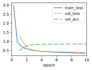
img_size, patch_size = 96, 16
num_hiddens, mlp_num_hiddens, num_heads, num_blks = 512, 2048, 8, 2
emb_dropout, blk_dropout, lr = 0.1, 0.1, 0.1
model = ViT(img_size, patch_size, num_hiddens, mlp_num_hiddens, num_heads,
            num_blks, emb_dropout, blk_dropout, lr)
trainer = d2l.Trainer(max_epochs=10, num_gpus=1)
data = d2l.FashionMNIST(batch_size=128, resize=(img_size, img_size))
trainer.fit(model, data)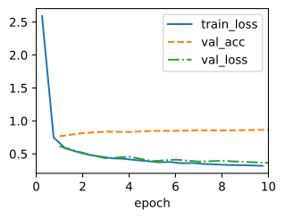
if tab.selected('pytorch'):
    vit_params = sum(p.numel() for p in model.parameters()
                     if p.requires_grad)
if tab.selected('jax'):
    vit_params = sum(p.size for p in
                     jax.tree.leaves(nnx.state(model, nnx.Param)))
vit_acc = float(model.board.data['val_acc'][-1].y)
print(f'ViT: {vit_params/1e6:.1f}M parameters, '
      f'validation accuracy {vit_acc:.2f}')
ViT: 6.5M parameters, validation accuracy 0.86if tab.selected('pytorch'):
vit_params = sum(p.numel() for p in model.parameters()
if p.requires_grad)
if tab.selected('jax'):
vit_params = sum(p.size for p in
jax.tree.leaves(nnx.state(model, nnx.Param)))
vit_acc = float(model.board.data['val_acc'][-1].y)
print(f'ViT: {vit_params/1e6:.1f}M parameters, '
f'validation accuracy {vit_acc:.2f}')ViT: 6.5M parameters, validation accuracy 0.87The model trains without drama to a validation accuracy of about 86–87%. Keep that number in mind; we will shortly see what a CNN of the same size does with the same ten epochs.
11.5.4.2 Do the Position Embeddings Discover the Grid?
First, though, let us look inside. The position embeddings started as noise, and nothing in the training signal ever named a row or a column. In fully trained ViTs the embeddings famously end up reflecting the grid anyway: in the original paper’s analysis, each position’s embedding is most similar to the embeddings of its spatial neighbors, with clear row and column bands — two-dimensional structure induced by the data alone (Dosovitskiy et al. 2021). Does our small model already show this? For each of the 36 patch positions we take its embedding vector, compute its cosine similarity with the embeddings of all 36 positions, and reshape those similarities into the \(6 \times 6\) patch grid. Laying out the 36 resulting maps in the grid itself gives a picture in which position \((i, j)\) of the big grid shows how similar position \((i, j)\)’s embedding is to everywhere else’s.
P = model.pos_embedding[0, 1:].detach().cpu()  # (36, 512): drop the cls slot
P = P / P.norm(dim=1, keepdim=True)
sim = P @ P.T                                  # Pairwise cosine similarities
coords = torch.stack(torch.meshgrid(
    torch.arange(6), torch.arange(6), indexing='ij'), -1).reshape(36, 2)
dist = (coords[:, None] - coords[None]).abs().amax(-1)  # Chebyshev distance
print(f'mean cosine similarity: grid neighbors {sim[dist == 1].mean():.2f}, '
      f'distant positions {sim[dist >= 3].mean():.2f}')
d2l.show_heatmaps(sim.reshape(6, 6, 6, 6), xlabel='', ylabel='',
                  figsize=(5, 5), cmap='Reds')
mean cosine similarity: grid neighbors 0.05, distant positions -0.03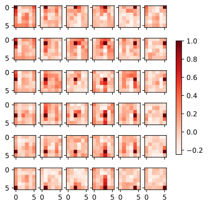
P = model.pos_embedding[0, 1:]                 # (36, 512): drop the cls slot
P = P / jnp.linalg.norm(P, axis=1, keepdims=True)
sim = P @ P.T                                  # Pairwise cosine similarities
coords = jnp.stack(jnp.meshgrid(
    jnp.arange(6), jnp.arange(6), indexing='ij'), -1).reshape(36, 2)
dist = jnp.abs(coords[:, None] - coords[None]).max(-1)  # Chebyshev distance
print(f'mean cosine similarity: grid neighbors {sim[dist == 1].mean():.2f}, '
      f'distant positions {sim[dist >= 3].mean():.2f}')
d2l.show_heatmaps(sim.reshape(6, 6, 6, 6), xlabel='', ylabel='',
                  figsize=(5, 5), cmap='Reds')
mean cosine similarity: grid neighbors 0.03, distant positions -0.02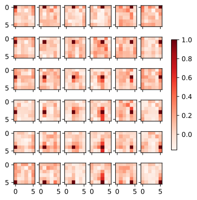
Each map’s darkest cell is its own position, which is mere self-similarity; the surrounding similarities determine whether spatial structure has emerged. After ten epochs, they show only weak traces of the grid. The printed statistic makes it precise: averaged over positions, immediate grid neighbors score slightly positive cosine similarity while distant positions score slightly negative, and several maps show a diffuse halo around their own cell or a weak band along their own column — but the values are small and the pattern is easy to miss without the summary statistics. Compare this with the crisp row-and-column structure that emerges in fully trained ViTs, and the state of our model is clear: the embeddings contain weak evidence of the spatial geometry that was not encoded at initialization. The next comparison uses an architecture that encodes this geometry directly.
11.5.4.3 A Convolutional Baseline at the Same Budget
The ViT above has about 6.5 million parameters. To make the inductive-bias comparison fair we build a CNN with the same budget, from the Residual blocks of Section 7.4: the familiar \(7 \times 7\) stem, then seven residual blocks whose channel widths are chosen so that the total lands at the ViT’s parameter count. It trains on the identical data pipeline for the identical ten epochs, with the learning rate that Section 7.4 established for this family.
class CompactResNet(d2l.Classifier):
    """A ResNet-style CNN parameter-matched to the ViT above."""
    def __init__(self, lr=0.01, num_classes=10):
        super().__init__()
        self.save_hyperparameters()
        self.net = nn.Sequential(
            nn.LazyConv2d(64, kernel_size=7, stride=2, padding=3),
            nn.LazyBatchNorm2d(), nn.ReLU(),
            nn.MaxPool2d(kernel_size=3, stride=2, padding=1),
            d2l.Residual(64), d2l.Residual(64),
            d2l.Residual(128, strides=2), d2l.Residual(128),
            d2l.Residual(256, strides=2), d2l.Residual(256),
            d2l.Residual(512, strides=2),
            nn.AdaptiveAvgPool2d((1, 1)), nn.Flatten(),
            nn.LazyLinear(num_classes))

    def forward(self, X):
        return self.net(X)
class CompactResNet(d2l.Classifier):
"""A ResNet-style CNN parameter-matched to the ViT above."""
def __init__(self, lr=0.01, num_classes=10, rngs=None):
super().__init__()
self.save_hyperparameters(ignore=['rngs'])
rngs = nnx.Rngs(0) if rngs is None else rngs
self.net = nnx.Sequential(
nnx.Conv(1, 64, kernel_size=(7, 7), strides=(2, 2),
padding='same', rngs=rngs),
nnx.BatchNorm(64, rngs=rngs), nnx.relu,
lambda x: nnx.max_pool(x, window_shape=(3, 3),
strides=(2, 2), padding='same'),
d2l.Residual(64, in_channels=64, rngs=rngs),
d2l.Residual(64, in_channels=64, rngs=rngs),
d2l.Residual(128, strides=(2, 2), in_channels=64, rngs=rngs),
d2l.Residual(128, in_channels=128, rngs=rngs),
d2l.Residual(256, strides=(2, 2), in_channels=128, rngs=rngs),
d2l.Residual(256, in_channels=256, rngs=rngs),
d2l.Residual(512, strides=(2, 2), in_channels=256, rngs=rngs),
lambda x: x.mean(axis=(1, 2)),
nnx.Linear(512, num_classes, rngs=rngs))
def forward(self, X):
return self.net(X)cnn = CompactResNet()
trainer = d2l.Trainer(max_epochs=10, num_gpus=1)
trainer.fit(cnn, data)
if tab.selected('pytorch'):
cnn_params = sum(p.numel() for p in cnn.parameters() if p.requires_grad)
if tab.selected('jax'):
cnn_params = sum(p.size for p in
jax.tree.leaves(nnx.state(cnn, nnx.Param)))
cnn_acc = float(cnn.board.data['val_acc'][-1].y)
print(f'CNN: {cnn_params/1e6:.1f}M parameters, '
f'validation accuracy {cnn_acc:.2f}')
print(f'ViT: {vit_params/1e6:.1f}M parameters, '
f'validation accuracy {vit_acc:.2f}')CNN: 6.5M parameters, validation accuracy 0.91
ViT: 6.5M parameters, validation accuracy 0.86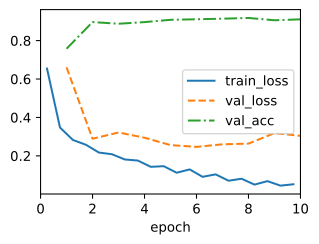
cnn = CompactResNet()
trainer = d2l.Trainer(max_epochs=10, num_gpus=1)
trainer.fit(cnn, data)
if tab.selected('pytorch'):
    cnn_params = sum(p.numel() for p in cnn.parameters() if p.requires_grad)
if tab.selected('jax'):
    cnn_params = sum(p.size for p in
                     jax.tree.leaves(nnx.state(cnn, nnx.Param)))
cnn_acc = float(cnn.board.data['val_acc'][-1].y)
print(f'CNN: {cnn_params/1e6:.1f}M parameters, '
      f'validation accuracy {cnn_acc:.2f}')
print(f'ViT: {vit_params/1e6:.1f}M parameters, '
      f'validation accuracy {vit_acc:.2f}')
CNN: 6.5M parameters, validation accuracy 0.91
ViT: 6.5M parameters, validation accuracy 0.87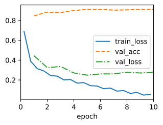
At the same parameter count, with the same data and number of epochs, the CNN performs better by several points, about 90–92% against the ViT’s 86–87%, a margin well beyond the run-to-run noise of these ten-epoch runs. The result is consistent with an advantage from the convolutional prior at this scale, although the comparison does not isolate that cause. Locality and translation equivariance are a strong prior the CNN has by construction; the transformer must infer both from data. After ten epochs, the position-embedding similarities show only weak grid structure. This experiment compares two models on Fashion-MNIST; it does not rank vision architectures generally. The discussion below considers published results under much larger pretraining protocols.
11.5.5 Summary
A vision transformer converts an image into a sequence with a strided convolution and processes the sequence with an encoder stack. Relative to the text model, the new components are the patch embedding, the “<cls>” readout, and learned position embeddings.
At matched parameter count, data, and training budget, the CNN performs better because convolution builds in locality and translation equivariance (Section 6.1), while the transformer must extract both from 60,000 images. Large-scale published comparisons reach a different outcome. Under the JFT-300M pretraining, model-size, and fine-tuning protocol of Dosovitskiy et al. (2021), ViT variants exceed the cited ResNet-based baselines. This result reflects the complete protocol, not data scale alone. DeiT showed that augmentation and distillation can make ViTs competitive on ImageNet-1k without JFT pretraining (Touvron et al. 2021). A complementary line, Swin transformers, reinstates convolution-like priors (local attention windows, hierarchical resolution) partly to escape the quadratic cost of global attention (Section 10.5) at high resolution (Liu et al. 2021).
Plain ViT encoders are used in several vision–language model families, including CLIP (Radford et al. 2021), while hierarchical transformers and convolutional backbones remain common in classification, detection, and segmentation. The appropriate backbone depends on the task, training protocol, and deployment constraints; Chapter 20 develops these applications.
11.5.6 Exercises
Parameters versus compute. The ViT of Section 11.5.4.1 reads grayscale images of \(h = w = 96\) pixels with \(c = 1\) channel through patches of side \(p = 16\). It has width \(d = 512\), MLP width \(4d\), and two blocks. Count one multiply–add as two FLOPs, as Equation 10.3.3 does, and write \(n = m + 1\) for the number of tokens.
- Express the parameter counts of
PatchEmbeddingand of the position embeddings as functions of \(p\). By how many parameters does the model change when \(p\) is halved to 8, and what fraction of its 6.5 million parameters is this change? - Show that the stem costs the same number of FLOPs per image for every \(p\). Derive the FLOPs of one
ViTBlockas a function of \(n\) and \(d\), and compute the factor by which the forward FLOPs of the model grow when \(p\) is halved to 8. - Find the number of tokens at which the term of your block count that is quadratic in \(n\) equals the remaining terms. Which patch sizes put this model beyond that point, and how far below it does ViT-B/16 operate, with \(d = 768\) at a resolution of \(224 \times 224\)?
CompactResNetwas matched to the ViT by parameter count. Count its convolution FLOPs per image, ignoring normalization, activations, and pooling, and compare them with those of the ViT. Is the comparison of Section 11.5.4.3 also matched in compute?
- Express the parameter counts of
[code] Patchify as convolution.
PatchEmbeddingreplaces cutting an image into patches and projecting each flattened patch by a single convolution whose kernel size and stride equal the patch size. Check this onpatch_embwith a batch of random images of its input shape. Cut the images into non-overlapping \(16 \times 16\) patches with reshapes and transpositions alone, flatten each patch, and apply the convolution’s kernel and bias, rearranged into a matrix and a vector. Verify that the result agrees with the output ofpatch_embup to floating-point round-off. In which order must the entries of a flattened patch appear, and in which order must the patches be enumerated?[code] Choice of readout.
ViTclassifies from the final representation of the “<cls>” token.- Under this readout, part of the computation of the last
ViTBlockcannot influence the logits. Identify it, and compute the fraction of the FLOPs of that block that inference could skip in the configuration of Section 11.5.4.1, counting as in problem 1. - Implement the alternative readout that averages the final representations of the 36 patches, and remove the “<cls>” token together with its position embedding. Train the model with the protocol of Section 11.5.4.1, and compare its validation accuracy with
vit_acc. - Dosovitskiy et al. (2021) report that the two readouts work about equally well but need different learning rates. Train both readouts at the learning rates \(0.03\) and \(0.3\) as well. Does the ranking of the two readouts depend on the learning rate?
- Under this readout, part of the computation of the last
[code] Position information. By the proposition of Section 10.4.1, self-attention without positional information is equivariant to permutations of its input tokens.
- Suppose that the 36 patch position embeddings of a
ViTare all equal. Show that its logits are then unchanged when the patch tokens are permuted, and that permuting the \(16 \times 16\) pixel blocks of the input image has the same effect as permuting the tokens. - Write a variant of
ViT.forwardthat applies a fixed permutation to the tokens produced byPatchEmbedding, before the position embeddings are added. Measure the validation accuracy of the trainedmodelunder five random permutations. - Train a
ViTwhose position embeddings are fixed at zero, with the protocol of Section 11.5.4.1. Compare its validation accuracy withvit_acc, and confirm that the five permutations leave its predictions unchanged. - Compare the accuracy drop under permutation with the gap between the two trained models. What does each of the two numbers measure?
- Suppose that the 36 patch position embeddings of a
[code] Grid permutation test. The two means printed in Section 11.5.4.2 compare the cosine similarity of the position embeddings of grid neighbors with that of distant positions. Let \(\Delta\) be their difference. Row \(k\) of
coordsholds the grid cell of the position embedding in row \(k\) ofP.- Pair the rows of
Pwith the rows ofcoordsthrough a random permutation, recompute \(\Delta\), and repeat 1,000 times. In what fraction of the permutations is \(\Delta\) at least as large as for the trainedmodel? What does this fraction say about the evidence for grid structure after ten epochs? - Train a
ViTwith the protocol of Section 11.5.4.1 for 30 epochs instead of 10, and repeat the test. How do \(\Delta\) and its position within the permutation distribution change with longer training?
- Pair the rows of
Shift equivariance. Shift a \(96 \times 96\) image by \(s\) pixels to the right, and fill the vacated columns with zeros. Suppose that the \(s\) rightmost columns of the original image are zero.
- For \(s = 16\), describe the tokens that
PatchEmbeddingproduces for the shifted image, and show that they are a rearrangement of those of the original image. Give an image for which this fails at \(s = 8\). - Use this and problem 4 to show that a
ViTwhose patch position embeddings are all equal assigns the same logits to both images when \(s = 16\). Why does the argument not extend to the trainedmodel? - Compute the stride of the final feature map of
CompactResNetrelative to its input. Show that, for cells whose receptive field lies inside the image, a shift of the input by a multiple of this stride moves the final feature map by whole cells, and explain why no such statement holds for a shift by fewer pixels. Compute the side length of the receptive field of a cell of the final feature map with Equation 6.2.3. Does any cell of the final feature map of a \(96 \times 96\) input meet the condition? - Neither model is therefore built to be invariant to a shift by one pixel. Name a property that every convolution of
CompactResNetbuilds in and the attention layers of the ViT lack, and a property that both models share.
- For \(s = 16\), describe the tokens that
[code] Higher resolution. ● Fine-tuning at a higher resolution than in pretraining keeps the patch size, so the grid of patches grows. Dosovitskiy et al. (2021) therefore interpolate the pretrained position embeddings in two dimensions to fit the new grid.
- Which parameters of
ViTdepend onimg_size? Explain why all others can be reused unchanged at a resolution of \(144 \times 144\). - Build a
ViTfor \(144 \times 144\) inputs and copy into it every parameter of the trainedmodelexcept the position embeddings. Keep the “<cls>” slot, and obtain the 81 patch position embeddings by reshaping the 36 trained ones into a \(6 \times 6 \times d\) array, resizing it bilinearly to \(9 \times 9 \times d\), and flattening it. Without further training, measure the validation accuracy on Fashion-MNIST resized to \(144 \times 144\). Compare it withvit_accand with the accuracy of the same model when all 81 patch embeddings equal the mean of the 36 trained ones. - Fine-tune the interpolated model for one epoch at \(144 \times 144\) with learning rate \(0.01\), and measure the time per epoch at both resolutions. Train a \(144 \times 144\)
ViTfrom scratch with the protocol of Section 11.5.4.1 for as many whole epochs as fit into the time of the ten epochs at \(96 \times 96\) plus the fine-tuning epoch. Compare the two accuracies. What does the comparison say about pretraining at low resolution?
- Which parameters of
[code] Recipe confound. ● Section 11.5.4.1 trains the ViT with the recipe of the convolutional networks of Chapter 7, plain SGD at a constant learning rate. Touvron et al. (2021) train ViTs on ImageNet-1k alone for 300 epochs, with AdamW, a cosine schedule, label smoothing, Mixup, and stronger augmentation.
- Retrain the ViT for 10 epochs with AdamW at weight decay \(0.05\) and the cosine schedule with warmup of Equation 7.6.2, using two warmup epochs and the base learning rates \(3 \times 10^{-4}\) and \(10^{-3}\). Compare the better of the two runs with
vit_accandcnn_acc. - Train the ViT with the better of the two settings, and
CompactResNetwith the optimizer of Section 11.5.4.3, for 30 epochs each, once plainly and once with Mixup at \(\alpha = 0.2\) (Equation 7.6.3) and label smoothing at \(\epsilon = 0.1\) (Equation 7.6.1). Tabulate the four validation accuracies. - The runs of the first two parts change three things in turn: the optimizer and schedule of the ViT, the training length from 10 to 30 epochs, and Mixup with label smoothing. Starting from the gap of Section 11.5.4.3, compute the gap between
CompactResNetand the ViT after each change. How much of the gap does each change close, and how large is the part that remains attributable to the architecture under the final protocol?
- Retrain the ViT for 10 epochs with AdamW at weight decay \(0.05\) and the cosine schedule with warmup of Equation 7.6.2, using two warmup epochs and the base learning rates \(3 \times 10^{-4}\) and \(10^{-3}\). Compare the better of the two runs with
Shifted windows. ● Swin transformers (Liu et al. 2021) restrict attention to non-overlapping windows of \(M \times M\) patches. Successive blocks alternate between a regular partition of the patch grid into windows and a partition displaced by \(\lfloor M/2 \rfloor\) patches along both axes. Normalization and MLPs act on each token separately. Call the set of input patches that can influence the output of a token after \(L\) blocks its reach. A window is the product of a row interval and a column interval, so the reach is the product of its one-dimensional counterparts, and it suffices to study one row of patches far from the border of the grid.
- Show that without the displaced partition, the reach of every token remains its own window at every depth.
- Show that with the alternation, the reach after \(L\) blocks is an interval of \(ML\) patches. Compare this growth with that of a stack of \(3 \times 3\) convolutions of stride 1 and with a single layer of global attention. On a \(56 \times 56\) grid with \(M = 7\), after how many blocks can the token in row 28 and column 28, counting from 0, be influenced by every patch?
- Show that the length \(ML\) stays the same for every displacement \(s\) with \(0 < s < M\). After two blocks, let \(g(s)\) be the smallest distance from a token to the nearer end of its reach, taken over all tokens. Compute \(g(s)\), and show that \(s = \lfloor M/2 \rfloor\) maximizes it.
[extended] Distillation from the CNN. ● Knowledge distillation trains a student model to match the predictions of a trained teacher model as well as the labels (Hinton et al. 2015). Touvron et al. (2021) find that ViTs distilled from a convolutional teacher outperform ViTs distilled from a transformer teacher, and suggest that the student inherits the inductive bias of the teacher. Use the trained
cnnas the teacher and a freshViTas the student. Let \(\mathbf{z}_s\) and \(\mathbf{z}_t\) be the logits of student and teacher for an image with label \(y\), let \(\mathrm{CE}\) be the cross-entropy of the softmax of its first argument, and let \(y_t\) be the class with the largest teacher logit. Hard-label distillation minimizes\[\mathcal{L}_\textrm{hard} = \tfrac{1}{2}\,\mathrm{CE}(\mathbf{z}_s, y) + \tfrac{1}{2}\,\mathrm{CE}(\mathbf{z}_s, y_t), \tag{11.5.1}\]
and soft distillation at temperature \(\tau\) and weight \(\lambda\) minimizes
\[\mathcal{L}_\textrm{soft} = (1 - \lambda)\,\mathrm{CE}(\mathbf{z}_s, y) + \lambda \tau^2\, \mathrm{KL}\big(\mathrm{softmax}(\mathbf{z}_t / \tau) \,\|\, \mathrm{softmax}(\mathbf{z}_s / \tau)\big). \tag{11.5.2}\]
- Compute the teacher’s logits on all training images once, and deliver them with each minibatch, so that the training step of the student needs no forward pass of the teacher. On what fraction of the training images is \(y_t \neq y\)? Explain what this fraction implies for the difference between \(\mathcal{L}_\textrm{hard}\) and plain cross-entropy in this setting, and why the implication does not carry over to the augmented training of Touvron et al. (2021).
- Override
training_stepofViTto minimize \(\mathcal{L}_\textrm{hard}\), and train with the protocol of Section 11.5.4.1. Train again with \(\mathcal{L}_\textrm{soft}\) at \(\tau = 3\) for \(\lambda \in \{0.1, 0.5\}\), and compare the three students withvit_acc. - For the undistilled
modeland for each student, compute the fraction of validation images on which its prediction differs from the teacher’s, as in the disagreement analysis of Touvron et al. (2021). Among the validation images that it misclassifies, compute also the fraction on which it predicts the same wrong class as the teacher. Which of the two numbers separates resemblance to the teacher from accuracy? - The teacher is both more accurate than the student and convolutional, so a gain from distillation does not by itself show that an inductive bias was transferred. Construct a control that separates the two explanations, run it, and state which outcome would favor the inductive-bias explanation.
[code] Attention distance. ● For one head, let \(\alpha_{ij}\) be the attention weight of query patch \(i\) on key patch \(j\) in an image, and let \(\mathbf{u}_i\) be the pixel coordinates of the center of patch \(i\). The mean attention distance of the head (Dosovitskiy et al. 2021) averages
\[\bar{r} = \frac{1}{36} \sum_{i=1}^{36} \sum_{j=1}^{36} \frac{\alpha_{ij}}{\sum_{k=1}^{36} \alpha_{ik}}\, \|\mathbf{u}_i - \mathbf{u}_j\| \tag{11.5.3}\]
over images, with the “<cls>” token excluded as query and key. In large pretrained ViTs, some heads of the lowest layers attend locally while others attend across the whole image, and the distance grows with depth.
- Evaluate \(\bar{r}\) for a head that attends uniformly to all 36 patches, as a reference value.
- After a forward pass of the trained
modelin evaluation mode,blk.attention.attention.attention_weightsholds the attention weights of blockblk, of shape (batch size \(\times\) 8, 37, 37), with the eight heads of each image adjacent. Compute \(\bar{r}\) for each of the 16 heads on 512 validation images, and plot it against the block index. Do the two blocks show either pattern of the pretrained ViTs? - Repeat the measurement for the ViT of problem 4 whose position embeddings are fixed at zero. What other than position embeddings can make a head attend to nearby patches, and how do the results of the two models separate the two causes?
[code] Attention distance. ● For one head, let \(\alpha_{ij}\) be the attention weight of query patch \(i\) on key patch \(j\) in an image, and let \(\mathbf{u}_i\) be the pixel coordinates of the center of patch \(i\). The mean attention distance of the head (Dosovitskiy et al. 2021) averages
\[\bar{r} = \frac{1}{36} \sum_{i=1}^{36} \sum_{j=1}^{36} \frac{\alpha_{ij}}{\sum_{k=1}^{36} \alpha_{ik}}\, \|\mathbf{u}_i - \mathbf{u}_j\| \tag{11.5.4}\]
over images, with the “<cls>” token excluded as query and key. In large pretrained ViTs, some heads of the lowest layers attend locally while others attend across the whole image, and the distance grows with depth.
- Evaluate \(\bar{r}\) for a head that attends uniformly to all 36 patches, as a reference value.
ViTBlock.__call__discards the attention weights thatd2l.MultiHeadAttentionreturns as its second output. Write a function that runs the trainedmodelasViT.forwarddoes, in deterministic mode, and also returns the weights of each block, of shape (batch size \(\times\) 8, 37, 37), with the eight heads of each image adjacent. Compute \(\bar{r}\) for each of the 16 heads on 512 validation images, and plot it against the block index. Do the two blocks show either pattern of the pretrained ViTs?- Repeat the measurement for the ViT of problem 4 whose position embeddings are fixed at zero. What other than position embeddings can make a head attend to nearby patches, and how do the results of the two models separate the two causes?