from d2l import torch as d2l
import torch3.4 Softmax Regression Implementation from Scratch
This section implements the components specific to softmax regression: the softmax transformation, cross-entropy loss, parameters, and forward pass. The data and training loop reuse the abstractions introduced for linear regression, making the differences between regression and classification explicit.
from d2l import tensorflow as d2l
import tensorflow as tf
from d2l import jax as d2l
from flax import nnx
import jax
from jax import numpy as jnpfrom d2l import mxnet as d2l
from mxnet import autograd, np, npx, gluon
npx.set_np()3.4.1 The Softmax
We begin with the transformation from scores to probabilities. Softmax normalizes each row of a matrix, so we will need per-row sums; recall from Section 1.3.2.2 and Section 1.3.2.3 how axis selects the dimension a sum collapses and keepdims preserves it for broadcasting:
X = d2l.tensor([[1.0, 2.0, 3.0], [4.0, 5.0, 6.0]])
d2l.reduce_sum(X, 0, keepdims=True), d2l.reduce_sum(X, 1, keepdims=True)(tensor([[5., 7., 9.]]),
tensor([[ 6.],
[15.]]))(<tf.Tensor: shape=(1, 3), dtype=float32, numpy=array([[5., 7., 9.]], dtype=float32)>,
<tf.Tensor: shape=(2, 1), dtype=float32, numpy=
array([[ 6.],
[15.]], dtype=float32)>)(Array([[5., 7., 9.]], dtype=float32),
Array([[ 6.],
[15.]], dtype=float32))(array([[5., 7., 9.]]),
array([[ 6.],
[15.]]))Computing the softmax requires three steps: (i) exponentiation of each term; (ii) a sum over each row to compute the normalization constant for each example; (iii) division of each row by its normalization constant, ensuring that the result sums to 1:
\[\mathrm{softmax}(\mathbf{X})_{ij} = \frac{\exp(\mathbf{X}_{ij})}{\sum_k \exp(\mathbf{X}_{ik})}. \tag{3.4.1}\]
The (logarithm of the) denominator is called the (log) partition function. It was introduced in statistical physics to sum over all possible states in a thermodynamic ensemble. The implementation is straightforward:
def softmax(X):
    X_exp = d2l.exp(X)
    partition = d2l.reduce_sum(X_exp, 1, keepdims=True)
    return X_exp / partition  # The broadcasting mechanism is applied here
For any input X, we turn each element into a nonnegative number. Each row sums up to 1, as is required for a probability. Caution: the code above is not robust against very large or very small arguments. While it is sufficient to illustrate what is happening, you should not use this code verbatim for any serious purpose. Deep learning frameworks have such protections built in and we will be using the built-in softmax going forward.
To see the failure rather than just assert it, feed in a logit that is large on the scale of \(\exp\). A score of \(1000\) overflows exp to infinity in float32, so the naive ratio becomes \(\infty/\infty\), which evaluates to NaN. The framework’s softmax subtracts the per-row maximum before exponentiating (the log-sum-exp trick of Section 3.5.2) and returns a finite distribution on exactly the same input:
z = torch.tensor([1000., 0., 0.])
naive = torch.exp(z) / torch.exp(z).sum()  # exp(1000) overflows -> nan
stable = torch.softmax(z, dim=0)           # built-in uses the log-sum-exp trick
naive, stable
(tensor([nan, 0., 0.]), tensor([1., 0., 0.]))z = tf.constant([1000., 0., 0.])
naive = tf.exp(z) / tf.reduce_sum(tf.exp(z)) # exp(1000) overflows -> nan
stable = tf.nn.softmax(z, axis=0) # built-in uses the log-sum-exp trick
naive, stable(<tf.Tensor: shape=(3,), dtype=float32, numpy=array([nan, 0., 0.], dtype=float32)>,
<tf.Tensor: shape=(3,), dtype=float32, numpy=array([1., 0., 0.], dtype=float32)>)z = jnp.array([1000., 0., 0.])
naive = jnp.exp(z) / jnp.exp(z).sum() # exp(1000) overflows -> nan
stable = jax.nn.softmax(z, axis=0) # built-in uses the log-sum-exp trick
naive, stable(Array([nan, 0., 0.], dtype=float32), Array([1., 0., 0.], dtype=float32))z = np.array([1000., 0., 0.])
naive = np.exp(z) / np.exp(z).sum() # exp(1000) overflows -> nan
stable = npx.softmax(z, axis=0) # built-in uses the log-sum-exp trick
naive, stable(array([nan, 0., 0.]), array([1., 0., 0.]))X = d2l.rand((2, 5))
X_prob = softmax(X)
X_prob, d2l.reduce_sum(X_prob, 1)(tensor([[0.1487, 0.2466, 0.1683, 0.2644, 0.1720],
[0.1916, 0.1833, 0.2432, 0.2470, 0.1350]]),
tensor([1., 1.]))X = d2l.rand((2, 5))
X_prob = softmax(X)
X_prob, d2l.reduce_sum(X_prob, 1)(<tf.Tensor: shape=(2, 5), dtype=float32, numpy=
array([[0.21319394, 0.13474208, 0.20669897, 0.17184985, 0.27351508],
[0.18383098, 0.17291924, 0.17053534, 0.20444588, 0.26826856]],
dtype=float32)>,
<tf.Tensor: shape=(2,), dtype=float32, numpy=array([0.9999999, 1. ], dtype=float32)>)X = jax.random.uniform(d2l.get_key(), (2, 5))
X_prob = softmax(X)
X_prob, d2l.reduce_sum(X_prob, 1)(Array([[0.15490438, 0.15702507, 0.27504665, 0.22082093, 0.19220296],
[0.14286114, 0.14374252, 0.23495987, 0.13943408, 0.33900243]], dtype=float32),
Array([1., 1.], dtype=float32))X = d2l.rand(2, 5)
X_prob = softmax(X)
X_prob, d2l.reduce_sum(X_prob, 1)(array([[0.21704897, 0.24554421, 0.24123886, 0.12218714, 0.17398085],
[0.19595093, 0.17780103, 0.22065419, 0.27965066, 0.12594323]]),
array([1., 1.]))3.4.2 The Model
We now have everything that we need to implement the softmax regression model. As in our linear regression example, each instance will be represented by a fixed-length vector. Since the raw data here consists of \(28 \times 28\) pixel images, we flatten each image, treating them as vectors of length 784. In later chapters, we will introduce convolutional neural networks, which exploit the spatial structure in a more satisfying way.
In softmax regression, the number of outputs from our network should be equal to the number of classes. Since our dataset has 10 classes, our network has an output dimension of 10. Consequently, our weights constitute a \(784 \times 10\) matrix plus a \(1 \times 10\) row vector for the biases. As with linear regression, we initialize the weights W with Gaussian noise. The biases are initialized as zeros.
class SoftmaxRegressionScratch(d2l.Classifier):
    def __init__(self, num_inputs, num_outputs, lr, sigma=0.01):
        super().__init__()
        self.save_hyperparameters()
        self.W = torch.normal(0, sigma, size=(num_inputs, num_outputs),
                              requires_grad=True)
        self.b = torch.zeros(num_outputs, requires_grad=True)

    def parameters(self):
        return [self.W, self.b]
class SoftmaxRegressionScratch(d2l.Classifier):
def __init__(self, num_inputs, num_outputs, lr, sigma=0.01):
super().__init__()
self.save_hyperparameters()
self.W = tf.random.normal((num_inputs, num_outputs), 0, sigma)
self.b = tf.zeros(num_outputs)
self.W = tf.Variable(self.W)
self.b = tf.Variable(self.b)class SoftmaxRegressionScratch(d2l.Classifier):
def __init__(self, num_inputs, num_outputs, lr, sigma=0.01, rngs=None):
super().__init__()
self.save_hyperparameters(ignore=['rngs'])
rngs = nnx.Rngs(d2l.get_key()) if rngs is None else rngs
self.W = nnx.Param(
rngs.params.normal((num_inputs, num_outputs)) * sigma)
self.b = nnx.Param(jnp.zeros(num_outputs))class SoftmaxRegressionScratch(d2l.Classifier):
def __init__(self, num_inputs, num_outputs, lr, sigma=0.01):
super().__init__()
self.save_hyperparameters()
self.W = np.random.normal(0, sigma, (num_inputs, num_outputs))
self.b = np.zeros(num_outputs)
self.W.attach_grad()
self.b.attach_grad()
def collect_params(self):
return [self.W, self.b]The code below defines how the network maps each input to an output. Note that we flatten each \(28 \times 28\) pixel image in the batch into a vector using reshape before passing the data through our model.
@d2l.add_to_class(SoftmaxRegressionScratch)
def forward(self, X):
    X = d2l.reshape(X, (-1, self.W.shape[0]))
    return softmax(d2l.matmul(X, self.W) + self.b)
3.4.3 The Cross-Entropy Loss
Next we need to implement the cross-entropy loss function (introduced in Section 3.1.3). This may be the most common loss function in deep-learning classification. Recall from Section 3.1.3 that minimizing cross-entropy is equivalent to maximizing the log-likelihood of the correct labels under our categorical model. It is the natural loss for classification. At the moment, applications of deep learning easily cast as classification problems far outnumber those better treated as regression problems.
Recall that cross-entropy takes the negative log-likelihood of the predicted probability assigned to the true label. For efficiency we avoid Python for-loops and use indexing instead. In particular, we select the correct-class probability for each row of \(\hat{\mathbf{y}}\) (equivalent to a dot product with the one-hot label).
To see this in action we create sample data y_hat with 2 examples of predicted probabilities over 3 classes and their corresponding labels y. The correct labels are \(0\) and \(2\) respectively (i.e., the first and third class). Using y as the indices of the probabilities in y_hat, we can pick out terms efficiently.
y = d2l.tensor([0, 2])
y_hat = d2l.tensor([[0.1, 0.3, 0.6], [0.3, 0.2, 0.5]])
y_hat[[0, 1], y]
tensor([0.1000, 0.5000])y_hat = tf.constant([[0.1, 0.3, 0.6], [0.3, 0.2, 0.5]])
y = tf.constant([0, 2])
tf.gather(y_hat, y, batch_dims=1)<tf.Tensor: shape=(2,), dtype=float32, numpy=array([0.1, 0.5], dtype=float32)>y = d2l.tensor([0, 2])
y_hat = d2l.tensor([[0.1, 0.3, 0.6], [0.3, 0.2, 0.5]])
y_hat[[0, 1], y]Array([0.1, 0.5], dtype=float32)y = d2l.tensor([0, 2])
y_hat = d2l.tensor([[0.1, 0.3, 0.6], [0.3, 0.2, 0.5]])
y_hat[[0, 1], y]array([0.1, 0.5])Now we can implement the cross-entropy loss function by averaging over the logarithms of the selected probabilities.
Now we can implement the cross-entropy loss function by averaging over the logarithms of the selected probabilities.
Now we can implement the cross-entropy loss function by averaging over the logarithms of the selected probabilities.
Note that to make use of jax.jit to speed up JAX implementations, and to make sure loss is a pure function, the cross_entropy function is re-defined inside the loss to avoid usage of any global variables or functions which may render the loss function impure. We refer interested readers to the JAX documentation on jax.jit and pure functions.
Now we can implement the cross-entropy loss function by averaging over the logarithms of the selected probabilities.
def cross_entropy(y_hat, y):
    # Tiny clip to keep log finite when softmax outputs underflow to 0.
    p = y_hat[list(range(len(y_hat))), y].clamp(min=1e-12)
    return -d2l.reduce_mean(d2l.log(p))

cross_entropy(y_hat, y)tensor(1.4979)def cross_entropy(y_hat, y):
p = tf.gather(y_hat, y, batch_dims=1)
# Tiny clip to keep log finite when softmax outputs underflow to 0.
return -tf.reduce_mean(tf.math.log(tf.maximum(p, 1e-12)))
cross_entropy(y_hat, y)<tf.Tensor: shape=(), dtype=float32, numpy=1.497866153717041>def cross_entropy(y_hat, y):
# Tiny clip to keep log finite when softmax outputs underflow to 0.
p = jnp.clip(jnp.take_along_axis(y_hat, jnp.expand_dims(y, -1),
axis=1).squeeze(-1), min=1e-12)
return -d2l.reduce_mean(d2l.log(p))
cross_entropy(y_hat, y)Array(1.4978662, dtype=float32)def cross_entropy(y_hat, y):
# Tiny clip to keep log finite when softmax outputs underflow to 0.
p = y_hat[list(range(len(y_hat))), y].clip(min=1e-12)
return -d2l.reduce_mean(d2l.log(p))
cross_entropy(y_hat, y)array(1.4978662)Note that we clip \(\hat{y}\) away from zero before taking \(\log\). Without the clip, \(\log(\hat{y})\) produces \(-\infty\) (and downstream NaNs) whenever the softmax assigns probability exactly zero to the correct class. Production code typically uses a log-softmax layer that fuses the softmax and log into a single numerically stable operation; the explicit clamp here is the minimal change that keeps the scratch implementation usable as a teaching example without changing its mathematical form. The proper fix, fusing softmax and cross-entropy via the log-sum-exp trick, is derived in Section 3.5.2.
@d2l.add_to_class(SoftmaxRegressionScratch)
def loss(self, y_hat, y):
return cross_entropy(y_hat, y)@d2l.add_to_class(SoftmaxRegressionScratch)
def loss(self, y_hat, y):
return cross_entropy(y_hat, y)@d2l.add_to_class(SoftmaxRegressionScratch)
def loss(self, y_hat, y):
return cross_entropy(y_hat, y)@d2l.add_to_class(SoftmaxRegressionScratch)
def loss(self, y_hat, y):
return cross_entropy(y_hat, y)3.4.4 Training
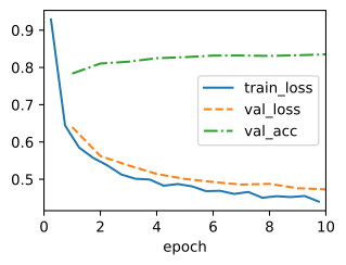
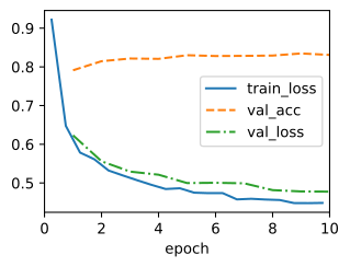
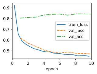
We reuse the fit method defined in Section 2.4 to train the model with 10 epochs. Note that the number of epochs (max_epochs), the minibatch size (batch_size), and learning rate (lr) are adjustable hyperparameters. That means that while these values are not learned during our primary training loop, they still influence the performance of our model, affecting both training and generalization. In practice you will want to choose these values based on the validation split of the data and then, ultimately, to evaluate your final model on the test split. As discussed in Section 2.6.3, we will regard the test data of Fashion-MNIST as the validation set, thus reporting validation loss and validation accuracy on this split.
data = d2l.FashionMNIST(batch_size=256)
model = SoftmaxRegressionScratch(num_inputs=784, num_outputs=10, lr=0.1)
trainer = d2l.Trainer(max_epochs=10)
trainer.fit(model, data)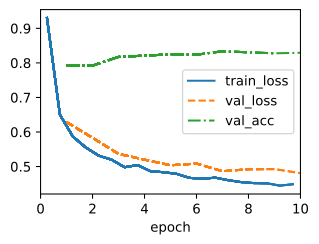
3.4.5 Prediction
Now that training is complete, our model is ready to classify some images.
X, y = next(iter(data.val_dataloader()))
with torch.no_grad():
    preds = d2l.argmax(model(X), axis=1)
preds.shapetorch.Size([256])X, y = next(iter(data.val_dataloader()))
preds = d2l.argmax(model(X), axis=1)
preds.shapeTensorShape([256])X, y = next(iter(data.val_dataloader()))
preds = d2l.argmax(model(X), axis=1)
preds.shape(256,)X, y = next(iter(data.val_dataloader()))
preds = d2l.argmax(model(X), axis=1)
preds.shape(256,)How well do we do overall? We sweep the whole validation set and average the per-example correct/incorrect flags returned by accuracy:
correct = []
for X_i, y_i in data.val_dataloader():
    with torch.no_grad():
        correct.append(model.accuracy(model(X_i), y_i, averaged=False))
print(f'Test accuracy: {torch.cat(correct).mean():.3f}')
Test accuracy: 0.823correct = []
for X_i, y_i in data.val_dataloader():
correct.append(model.accuracy(model(X_i), y_i, averaged=False))
print(f'Test accuracy: {float(tf.reduce_mean(tf.concat(correct, 0))):.3f}')Test accuracy: 0.834correct = []
for X_i, y_i in data.val_dataloader():
correct.append(model.accuracy(model(X_i), y_i, averaged=False))
print(f'Test accuracy: {float(jnp.concatenate(correct).mean()):.3f}')Test accuracy: 0.830correct = []
for X_i, y_i in data.val_dataloader():
correct.append(model.accuracy(model(X_i), y_i, averaged=False))
print(f'Test accuracy: {float(np.concatenate(correct).mean()):.3f}')Test accuracy: 0.833The overall test accuracy comes out at roughly 82–83% (the exact value varies a little from run to run), consistent with the training curve: the performance of this linear model on Fashion-MNIST. We are more interested in the images we label incorrectly. We visualize them by comparing their actual labels (first line of text output) with the predictions from the model (second line of text output).
wrong = d2l.astype(preds, y.dtype) != y
X, y, preds = X[wrong], y[wrong], preds[wrong]
labels = [a+'\n'+b for a, b in zip(
    data.text_labels(y), data.text_labels(preds))]
data.visualize([X, y], labels=labels)



The gallery shows which images fail; to see how they fail in aggregate we compute the confusion matrix Equation 3.3.2 introduced in Section 3.3. We accumulate a \(10\times10\) matrix of counts \(C\) over the validation set, with entry \((i, j)\) counting how often true class \(j\) was predicted as class \(i\), and then normalize each column,
\[\tilde{C}_{ij} = C_{ij} \Big/ \sum_{i'} C_{i'j}, \tag{3.4.2}\]
so that column \(j\) shows the distribution of predictions for class \(j\) (classes are indexed in the order of text_labels: t-shirt, trouser, pullover, dress, coat, sandal, shirt, sneaker, bag, ankle boot).
To display that matrix of counts as a grid of colored cells rather than a wall of numbers, we define show_heatmaps, a display utility we reuse throughout the book (e.g., for visualizing attention weights).
def show_heatmaps(matrices, xlabel, ylabel, titles=None, figsize=(2.5, 2.5),
                  cmap='Reds'):
    """Show heatmaps of matrices."""
    d2l.use_svg_display()
    num_rows, num_cols, _, _ = matrices.shape
    fig, axes = d2l.plt.subplots(num_rows, num_cols, figsize=figsize,
                                 sharex=True, sharey=True, squeeze=False)
    for i, (row_axes, row_matrices) in enumerate(zip(axes, matrices)):
        for j, (ax, matrix) in enumerate(zip(row_axes, row_matrices)):
            pcm = ax.imshow(d2l.numpy(matrix), cmap=cmap)
            if i == num_rows - 1:
                ax.set_xlabel(xlabel)
            if j == 0:
                ax.set_ylabel(ylabel)
            if titles:
                ax.set_title(titles[j])
    fig.colorbar(pcm, ax=axes, shrink=0.6);
def show_heatmaps(matrices, xlabel, ylabel, titles=None, figsize=(2.5, 2.5),
                  cmap='Reds'):
    """Show heatmaps of matrices."""
    d2l.use_svg_display()
    num_rows, num_cols, _, _ = matrices.shape
    fig, axes = d2l.plt.subplots(num_rows, num_cols, figsize=figsize,
                                 sharex=True, sharey=True, squeeze=False)
    for i, (row_axes, row_matrices) in enumerate(zip(axes, matrices)):
        for j, (ax, matrix) in enumerate(zip(row_axes, row_matrices)):
            pcm = ax.imshow(matrix, cmap=cmap)
            if i == num_rows - 1:
                ax.set_xlabel(xlabel)
            if j == 0:
                ax.set_ylabel(ylabel)
            if titles:
                ax.set_title(titles[j])
    fig.colorbar(pcm, ax=axes, shrink=0.6);
def show_heatmaps(matrices, xlabel, ylabel, titles=None, figsize=(2.5, 2.5),
                  cmap='Reds'):
    """Show heatmaps of matrices."""
    d2l.use_svg_display()
    num_rows, num_cols, _, _ = matrices.shape
    fig, axes = d2l.plt.subplots(num_rows, num_cols, figsize=figsize,
                                 sharex=True, sharey=True, squeeze=False)
    for i, (row_axes, row_matrices) in enumerate(zip(axes, matrices)):
        for j, (ax, matrix) in enumerate(zip(row_axes, row_matrices)):
            pcm = ax.imshow(d2l.numpy(matrix), cmap=cmap)
            if i == num_rows - 1:
                ax.set_xlabel(xlabel)
            if j == 0:
                ax.set_ylabel(ylabel)
            if titles:
                ax.set_title(titles[j])
fig.colorbar(pcm, ax=axes, shrink=0.6);C = torch.zeros(10, 10)
for X_i, y_i in data.val_dataloader():
with torch.no_grad():
preds_i = model(X_i).argmax(axis=1)
C += torch.bincount(10 * preds_i + y_i, minlength=100).reshape(10, 10)
C /= C.sum(axis=0, keepdims=True) # column j: true class j
d2l.show_heatmaps(C.reshape(1, 1, 10, 10), xlabel='true class',
ylabel='predicted class', figsize=(3.5, 3.5), cmap='Blues')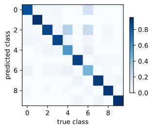
C = tf.zeros((10, 10), dtype=tf.int32)
for X_i, y_i in data.val_dataloader():
    preds_i = tf.cast(d2l.argmax(model(X_i), axis=1), y_i.dtype)
    C += tf.transpose(tf.math.confusion_matrix(y_i, preds_i, num_classes=10))
C = tf.cast(C, tf.float32)
C /= tf.reduce_sum(C, axis=0, keepdims=True)   # column j: true class j
d2l.show_heatmaps(tf.reshape(C, (1, 1, 10, 10)), xlabel='true class',
                  ylabel='predicted class', figsize=(3.5, 3.5), cmap='Blues')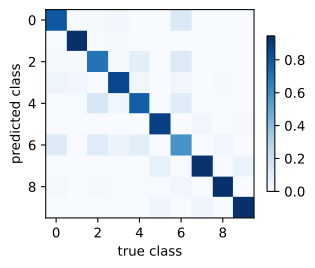
C = jnp.zeros((10, 10))
for X_i, y_i in data.val_dataloader():
    preds_i = d2l.argmax(model(X_i), axis=1)
    C += jnp.bincount(10 * preds_i + y_i, length=100).reshape(10, 10)
C /= C.sum(axis=0, keepdims=True)              # column j: true class j
d2l.show_heatmaps(C.reshape(1, 1, 10, 10), xlabel='true class',
                  ylabel='predicted class', figsize=(3.5, 3.5), cmap='Blues')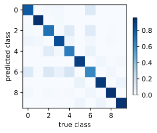
C = np.zeros((10, 10))
for X_i, y_i in data.val_dataloader():
    preds_i = model(X_i).argmax(axis=1).asnumpy()
    for i, j in zip(preds_i, y_i.asnumpy()):
        C[int(i), int(j)] += 1
C /= C.sum(axis=0, keepdims=True)              # column j: true class j
d2l.show_heatmaps(C.reshape(1, 1, 10, 10), xlabel='true class',
                  ylabel='predicted class', figsize=(3.5, 3.5), cmap='Blues')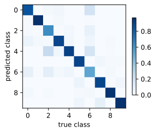
The errors concentrate in two groups. Upper-body garments (t-shirt, pullover, dress, coat, shirt: columns 0, 2, 3, 4, 6) trade errors almost exclusively among themselves, and the shirt column has the largest off-diagonal mass, with predictions often assigned to t-shirt, pullover, and coat; footwear (sandal, sneaker, ankle boot: columns 5, 7, 9) forms a second, smaller cluster. Meanwhile, trousers and bags have predominantly diagonal entries, indicating fewer errors for this fitted linear model. This makes the summary’s claim visible, since to a classifier that can only weigh pixels linearly, garments with similar global pixel patterns, such as shirts and pullovers, can be difficult to distinguish, while classes that differ in silhouette are easy.
3.4.6 Summary and Discussion
In this section we built softmax regression from its constituent operations: softmax, cross-entropy, parameter initialization, the forward pass, and the optimization step. The concise implementation in Section 3.5 packages the same computation into framework primitives, including a fused and numerically stable loss.
What this training curve shows. In the displayed run, 10 epochs of minibatch SGD reach roughly 82–83% validation accuracy. The confusion matrix shows that many remaining errors involve upper-body garments with similar pixel patterns. This observation diagnoses the fitted model; it does not establish a universal accuracy ceiling for linear classifiers or rule out improvements from different preprocessing, optimization, or regularization.
Why clipping is incomplete. The clip stops \(\log 0\) but leaves the naive softmax free to overflow for large logits; the stable approach (subtracting the row maximum before exponentiating and fusing softmax with log) is derived in Section 3.5.2, which the concise implementation applies automatically.
3.4.7 Exercises
[code] Numerical stability. The
softmaxof this section returnsNaNon a matrix whose single row is the logits \((1000, 0, 0)\), because \(\exp(1000)\) overflows.- Show that it also returns
NaNon the row \((-1000, -1000, -1000)\), and identify the operation that produces theNaNin this case. - Implement a fix that subtracts the largest entry of each row before exponentiating, and check that it agrees with the built-in softmax on both rows and on random inputs.
- Show that it also returns
[code] Cross-entropy from one-hot labels. The
cross_entropyof this section selects the correct-class probability by indexing. Implement an alternative that follows the definition \(-\sum_j y_j \log \hat{y}_j\) literally, by convertingyto a one-hot matrix and taking row-wise inner products.- Use it as the
lossofSoftmaxRegressionScratchand confirm that training is unchanged. - Time both versions on random probability matrices with \(256\) rows and \(q \in \{10, 10^3, 10^5\}\) columns, and state how the memory that each version allocates grows with \(q\).
- Describe a setting in which the inner-product form applies but the indexing form does not.
- Use it as the
Large vocabularies. Suppose that softmax regression predicts the next word from a feature vector of dimension \(d = 1024\). The vocabulary has \(V = 10^6\) words, and each minibatch holds \(n = 256\) examples. List the operations of
forwardandcross_entropywhose cost grows with \(V\). Compute the multiply-adds of the matrix product, the float32 memory ofW, and the float32 memory of the \(n \times V\) matrix of probabilities, and compare each number with the Fashion-MNIST model of this section.Output-layer gradients. ● Consider softmax regression that predicts the next word from a vocabulary of \(V = 10^6\) words. By Section 3.1.3.2, the derivative of the loss with respect to the logit \(o_j\) is \(\hat{y}_j - y_j\). Explain why a single example produces a nonzero gradient for every column of
W, and propose a change to the output layer that updates only a few columns per example.[code] Hyperparameter sweep. Retrain
SoftmaxRegressionScratchwithd2l.Trainer(max_epochs=10), varying one hyperparameter at a time.- Plot the final validation loss against the learning rate over \(\{0.01, 0.03, 0.1, 0.3, 1\}\).
- Plot the final training and validation losses against the minibatch size over \(\{8, 32, 256, 2048\}\) at learning rate \(0.1\).
- Compute the number of parameter updates that ten epochs over the 60,000 training images take at each batch size. Use these counts to explain the trend in the previous plot, and predict how the comparison changes when every run takes the same number of updates.
[code] Confusion matrix. The diagonal of the column-normalized confusion matrix Equation 3.4.2 holds the per-class recall.
- Compute the row-normalized counterpart, whose diagonal holds the per-class precision. Find the class whose precision and recall differ most, and state whether the model predicts that class more often or less often than it occurs.
- Reshape each column of the weight matrix
Winto a \(28 \times 28\) image and display the ten templates withshow_images. Relate visually similar templates to the most confused class pairs.
[code] ROC of the trained model. Exercises 6 and 7 of Section 3.3 define the ROC curve and the area under it (AUC) on simulated scores. Apply them to the trained
SoftmaxRegressionScratchon the validation images of two classes \(a\) and \(b\), with \(a\) as the positive class. Becauseforwardreturns probabilities rather than logits, use the score\[s = \frac{\hat{y}_a}{\hat{y}_a + \hat{y}_b},\]
which equals \(\sigma(o_a - o_b)\) by Equation 3.1.3.
- Plot the ROC curves and compute the AUCs for sneaker versus sandal and for shirt versus t-shirt.
- Compare the ordering of the two AUCs with the off-diagonal entries of the confusion matrix \(C\) for the same pairs, and explain why the two diagnostics need not agree.