from d2l import torch as d2l
import math
import torch
from torch import nn
from torch.nn import functional as F7.7 ConvNeXt: A ConvNet for the 2020s
By 2021, vision Transformers (Dosovitskiy et al. 2021) led the ImageNet leaderboard, and hierarchical variants such as the Swin Transformer (Liu et al. 2021) were increasingly used as backbones for detection and segmentation. These results raised the question of whether attention had superseded convolution. But a transformer differs from a 2015 ResNet in many ways besides attention: its training recipe, its stem, its activation function, its normalization layers, the shape and depth of its stages. Which of these differences actually carried the improvement?
Z. Liu et al. (2022) answered by experiment. Starting from a ResNet-50, they applied one transformer-inspired design change at a time, measured ImageNet accuracy, retained changes that helped, and did not add attention. The resulting ConvNeXt reaches 82.0% top-1 accuracy, compared with 81.3% for a Swin-T transformer of similar computational cost. The modifications use concepts introduced earlier: modern training procedures (Section 7.6), depthwise convolutions (Section 6.4.4), inverted bottlenecks (Section 7.5), receptive fields (Equation 6.2.3), and normalization layers (Section 7.3). We examine the ablation sequence, implement the architecture, and train a scaled-down ConvNeXt.
import tensorflow as tf
from d2l import tensorflow as d2l
from d2l import jax as d2l
from flax import nnx
import jax
from jax import numpy as jnp
import optaxfrom d2l import mxnet as d2l
import math
import mxnet as mx
from mxnet import gluon, init, np, npx
from mxnet.gluon import nn
npx.set_np()7.7.1 The Modernization Roadmap
Table 7.7.1 shows the full sequence. Each row keeps every change above it, so the accuracies are cumulative; the computational cost is held near that of Swin-T (about 4.5 GFLOPs) throughout.
| Change | What it means | Top-1 |
|---|---|---|
| (starting point) | ResNet-50 with its 2015 recipe | 76.1% |
| Modern training recipe | 300 epochs, AdamW, Mixup, label smoothing, stochastic depth (Section 7.6) | 78.8% |
| Stage ratio | blocks per stage \((3, 4, 6, 3) \to (3, 3, 9, 3)\) | 79.4% |
| Patchify stem | \(7 \times 7\) stride-2 convolution plus pooling \(\to\) one \(4 \times 4\) stride-4 convolution | 79.5% |
| Depthwise convolutions | the \(3 \times 3\) convolution becomes depthwise; width grows from 64 to 96 channels | 80.5% |
| Inverted bottleneck | expand \(4\times\) inside the block instead of compressing | 80.6% |
| Large kernels | depthwise convolution moved to the front and enlarged to \(7 \times 7\) | 80.6% |
| ReLU \(\to\) GELU | a smooth activation, as in transformers | 80.6% |
| Fewer activations | one activation per block instead of three | 81.3% |
| Fewer normalizations | one normalization per block instead of three | 81.4% |
| BN \(\to\) LN | layer normalization over channels at each position | 81.5% |
| Separate downsampling | an LN plus \(2 \times 2\) stride-2 convolution between stages | 82.0% |
The first row gives the largest single improvement without changing the architecture. The 2.7 points it contributes are the recipe effect of Section 7.6 (the “ResNet strikes back” study pushed the same network to 80.4% with a still longer 600-epoch procedure (Wightman et al. 2021)). Keep this split in mind for everything below: of the 5.9 points separating the 2015 ResNet-50 from ConvNeXt, 2.7 are training and 3.2 are architecture. Papers that compared a well-tuned transformer against a 2015-recipe ResNet were, in large part, comparing recipes.
7.7.1.1 Macro design
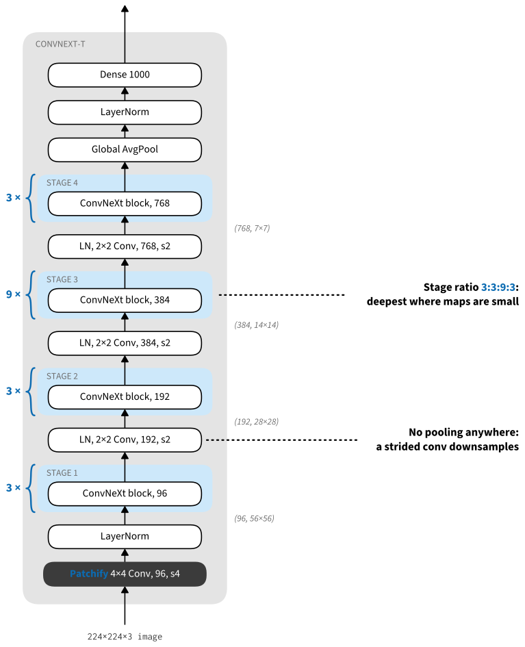
The next two rows change the network’s silhouette. Swin-T distributes its blocks across the four stages in the ratio \(1{:}1{:}3{:}1\), spending most of its depth where the feature maps are small and each block is cheap; adopting the same ratio turns ResNet-50’s \((3, 4, 6, 3)\) blocks into \((3, 3, 9, 3)\) and adds 0.6 points. The stem changes more. ResNet begins with a \(7 \times 7\) stride-2 convolution followed by max-pooling, a fourfold reduction computed with overlapping windows. Vision transformers instead slice the image into non-overlapping patches, which is equivalent to a strided convolution whose kernel size equals its stride (Section 6.3): a \(4 \times 4\) convolution with stride 4. This patchify stem replaces the ResNet stem with no loss (79.5%), and its output is the same object a transformer calls a patch embedding: one feature vector per \(4 \times 4\) patch.
7.7.1.2 Depthwise convolutions and the inverted bottleneck
The attention core of a transformer mixes information across positions using one weight pattern per head. Its query, key, value, and output projections also mix channels. The MLP that follows mixes channels independently at each position. MobileNet factorizes a convolution in a related way: a depthwise convolution mixes positions within each channel, then \(1 \times 1\) convolutions mix channels (Section 6.4.4). The ResNet bottleneck’s \(3 \times 3\) convolution therefore becomes depthwise, and the savings permit width (64 to 96 channels, matching Swin-T), which brings 80.5%. Inverting the bottleneck adds a little more (80.6%): the block now expands its thin residual stream by \(4\times\) and projects back. We saw in Section 7.5 why this shape is economical once the spatial convolution is depthwise. The transformer’s MLP uses the same factor-four pointwise expand–activate–project substructure; ConvNeXt adds the depthwise spatial mixer before it.
With the expensive dense convolution gone, kernel size stops being a luxury. The depthwise convolution moves to the front of the block, so that the cheap operation sees the unexpanded stream; this alone temporarily costs 0.7 points, and enlarging the kernel from \(3 \times 3\) to \(7 \times 7\) recovers the loss at lower cost. By Equation 6.2.3, a \(7 \times 7\) kernel grows the receptive field as fast as three stacked \(3 \times 3\) layers, the trade VGG once resolved in favor of depth (Section 7.2.1) when kernels were dense and their cost quadratic. Depthwise, a \(7 \times 7\) kernel costs only \(49/9 \approx 5\times\) a \(3 \times 3\) one on the depthwise term alone, a small fraction of the block. The authors report that accuracy saturates at \(7 \times 7\): kernels of \(9 \times 9\) and \(11 \times 11\) provide no further improvement at this scale.
7.7.1.3 Micro design
The remaining rows are small and, cumulatively, decisive. GELU is the smooth activation used in transformers and in essentially every large language model; replacing ReLU with it changes nothing by itself (80.6%). What matters is how many activations and normalizations the block contains. A ResNet bottleneck interleaves a normalization and an activation after every convolution: three of each. A transformer block applies one activation, inside its MLP, and one or two normalizations. Deleting all but one GELU (between the two \(1 \times 1\) convolutions) adds 0.7 points, more than any other micro-design change; deleting all but one normalization adds a little more, and swapping that survivor from batch normalization to layer normalization over the channels at each spatial position adds another tenth (81.5%). The lesson of Section 7.3 reappears: normalization is scaffolding for optimization, and less of it, placed well, can be better. Figure 7.7.1 shows the before and after.
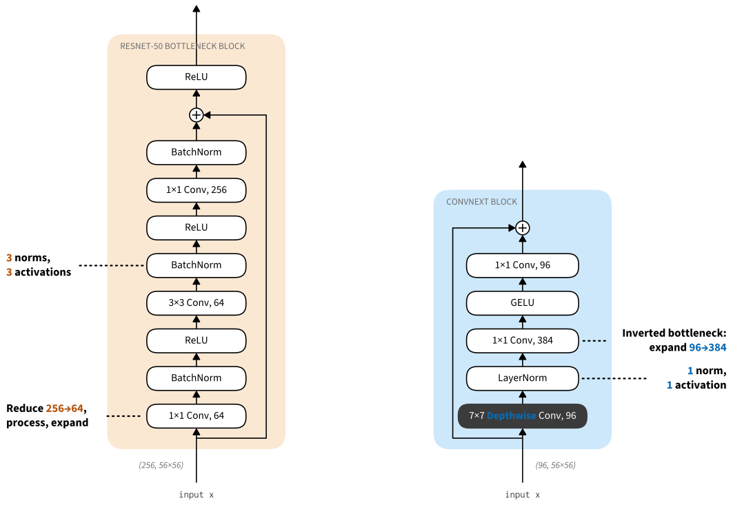
Finally, ResNet downsamples inside the first block of each stage, by giving its \(3 \times 3\) convolution a stride of 2. Swin instead uses a separate patch-merging layer between stages. Adopting the same separation completes the roadmap at 82.0%: a layer normalization followed by a \(2 \times 2\) stride-2 convolution between stages, plus a normalization after the stem and one before the classifier head, which the authors found necessary for stable training. Figure 7.7.2 shows the assembled ConvNeXt-T: a patchify stem, four stages of \((3, 3, 9, 3)\) blocks at widths \((96, 192, 384, 768)\), downsampling layers between them, and a global-average-pooling head, the stem-body-head layout this chapter has used since Section 7.2.3.
At this scale, the comparison is approximately even: a convolutional network using the Transformer’s training procedure and several related design choices matches or slightly exceeds the Transformer. The paper reports similar results for larger variants and for transfer to COCO detection and ADE20K segmentation, the discriminating benchmarks discussed in Section 7.6. These experiments demonstrate competitiveness, not an inherent advantage for convolution; under comparable tuning, the two families attain similar results. We return to what that means in Section 7.8.
7.7.2 Implementation
ConvNeXt is easy to build precisely because the roadmap removed things. A block is six operations; the network is the familiar arch-tuple loop.
7.7.2.1 The ConvNeXt block
The block applies, in order: a \(7 \times 7\) depthwise convolution, layer normalization, a \(1 \times 1\) convolution expanding the channels \(4\times\), a GELU, and a \(1 \times 1\) convolution projecting back, with the result added to the input. Two refinements from the paper’s training setup come along. Layer scale multiplies the branch by a learnable per-channel vector \(\gamma\) initialized to \(10^{-6}\), so every block starts as a near-identity and the network begins training as a shallow function that gradually deepens; the technique was introduced for very deep vision transformers (Touvron et al. 2021) and helps stability here too. Stochastic depth, Equation 7.6.4 of Section 7.6, randomly drops the whole branch per sample during training.
One implementation detail deserves attention: the layer-normalization placement that the roadmap’s LN row depends on. ConvNeXt normalizes over the channels at each spatial position, the same normalization a transformer applies to each token. In a channels-last layout (samples, height, width, channels) this is the library default, and a \(1 \times 1\) convolution is a linear layer applied to the last axis. Our PyTorch implementation therefore permutes to channels-last inside the block, while TensorFlow and JAX are channels-last natively. MXNet stays channels-first and normalizes axis=1.
The MXNet block implements the deterministic ConvNeXt transformation and layer scale. This reduced variant omits stochastic depth; PyTorch, JAX, and TensorFlow include the per-sample mask used for training.
def drop_path(Y, p, training):  # Stochastic depth, as in the previous section
    if not training or p == 0:
        return Y
    keep = (torch.rand(Y.shape[0], 1, 1, 1, device=Y.device) > p).float()
    return Y * keep / (1 - p)

class ConvNeXtBlock(nn.Module):
    """Depthwise 7x7, LN, 1x1 expand, GELU, 1x1 project, scaled residual."""
    def __init__(self, dim, drop_prob=0.0, layer_scale=1e-6):
        super().__init__()
        self.dwconv = nn.Conv2d(dim, dim, kernel_size=7, padding=3,
                                groups=dim)
        self.norm = nn.LayerNorm(dim, eps=1e-6)
        self.pwconv1 = nn.Linear(dim, 4 * dim)  # 1x1 conv in channels-last
        self.pwconv2 = nn.Linear(4 * dim, dim)
        self.gamma = nn.Parameter(layer_scale * torch.ones(dim))
        self.drop_prob = drop_prob

    def forward(self, X):
        Y = self.dwconv(X).permute(0, 2, 3, 1)  # to channels-last
        Y = self.pwconv2(F.gelu(self.pwconv1(self.norm(Y))))
        Y = (self.gamma * Y).permute(0, 3, 1, 2)  # back to channels-first
        return X + drop_path(Y, self.drop_prob, self.training)
class ConvNeXtBlock(tf.keras.layers.Layer):
"""Depthwise 7x7, LN, 1x1 expand, GELU, 1x1 project, scaled residual."""
def __init__(self, dim, drop_prob=0.0, layer_scale=1e-6):
super().__init__()
self.dwconv = tf.keras.layers.DepthwiseConv2D(kernel_size=7,
padding='same')
self.norm = tf.keras.layers.LayerNormalization(epsilon=1e-6)
self.pwconv1 = tf.keras.layers.Dense(4 * dim)
self.pwconv2 = tf.keras.layers.Dense(dim)
self.gamma = self.add_weight(
shape=(dim,),
initializer=tf.keras.initializers.Constant(layer_scale))
self.drop_prob = drop_prob
def call(self, X, training=False):
Y = self.norm(self.dwconv(X))
Y = self.pwconv2(tf.keras.activations.gelu(self.pwconv1(Y)))
Y = self.gamma * Y
if training and self.drop_prob > 0:
keep = tf.cast(tf.random.uniform((tf.shape(Y)[0], 1, 1, 1))
> self.drop_prob, Y.dtype)
Y = Y * keep / (1 - self.drop_prob)
return X + Yclass ConvNeXtBlock(nnx.Module):
"""Depthwise 7x7, LN, 1x1 expand, GELU, 1x1 project, scaled residual."""
deterministic: bool
def __init__(self, dim, drop_prob=0.0, layer_scale=1e-6, rngs=None):
rngs = (nnx.Rngs(params=d2l.get_key(), dropout=d2l.get_key())
if rngs is None else rngs)
self.dim, self.drop_prob = dim, drop_prob
self.deterministic = False
self.rngs = rngs
self.dwconv = nnx.Conv(dim, dim, kernel_size=(7, 7), padding='same',
feature_group_count=dim, rngs=rngs)
self.norm = nnx.LayerNorm(dim, epsilon=1e-6, rngs=rngs)
self.pwconv1 = nnx.Linear(dim, 4 * dim, rngs=rngs)
self.pwconv2 = nnx.Linear(4 * dim, dim, rngs=rngs)
self.gamma = nnx.Param(layer_scale * jnp.ones(dim))
def set_view(self, *, deterministic):
self.deterministic = deterministic
def __call__(self, X):
Y = self.norm(self.dwconv(X))
Y = self.pwconv2(nnx.gelu(self.pwconv1(Y)))
Y = self.gamma * Y
if not self.deterministic and self.drop_prob > 0:
keep = jax.random.bernoulli(
self.rngs.dropout(), 1 - self.drop_prob,
(X.shape[0], 1, 1, 1))
Y = Y * keep / (1 - self.drop_prob)
return X + Yclass ConvNeXtBlock(nn.Block):
"""Depthwise 7x7, LN, 1x1 expand, GELU, 1x1 project, scaled residual."""
def __init__(self, dim, layer_scale=1e-6):
super().__init__()
self.dwconv = nn.Conv2D(dim, kernel_size=7, padding=3, groups=dim)
self.norm = nn.LayerNorm(axis=1, epsilon=1e-6)
self.pwconv1 = nn.Conv2D(4 * dim, kernel_size=1)
self.act = nn.GELU()
self.pwconv2 = nn.Conv2D(dim, kernel_size=1)
self.gamma = gluon.Parameter('gamma', shape=(1, dim, 1, 1),
init=init.Constant(layer_scale))
def forward(self, X):
Y = self.norm(self.dwconv(X))
Y = self.pwconv2(self.act(self.pwconv1(Y)))
return X + self.gamma.data() * Y7.7.2.2 The full network
The network is the arch-tuple pattern of Section 7.2.1 one more time: a tuple of (depth, channels) pairs, a stem, a loop, a head. The stem is the patchify convolution plus a normalization. Between stages sits the separate downsampling layer, a normalization followed by a \(2 \times 2\) stride-2 convolution; there is no pooling anywhere in the body. Following the paper, the per-block stochastic-depth probability ramps linearly from zero at the first block to its maximum at the last. Our dimensions are a scaled-down ConvNeXt sized for Fashion-MNIST, near the “atto” end of the family: widths \((40, 80, 160, 320)\) and depths \((2, 2, 6, 2)\), with the third stage deepest as in the full model.
class LayerNorm2d(nn.LayerNorm):
    """LayerNorm over the channel axis of an NCHW tensor."""
    def forward(self, X):
        return super().forward(X.permute(0, 2, 3, 1)).permute(0, 3, 1, 2)

class ConvNeXt(d2l.Classifier):
    arch = ((2, 40), (2, 80), (6, 160), (2, 320))

    def __init__(self, lr=2e-3, num_classes=10, drop_path_max=0.1):
        super().__init__()
        self.save_hyperparameters()
        depths = [d for d, c in self.arch]
        rates = torch.linspace(0, drop_path_max, sum(depths)).tolist()
        layers = [nn.Conv2d(1, self.arch[0][1], kernel_size=4, stride=4),
                  LayerNorm2d(self.arch[0][1], eps=1e-6)]
        c_prev, b = self.arch[0][1], 0
        for i, (depth, c) in enumerate(self.arch):
            if i > 0:  # separate downsampling layer between stages
                layers += [LayerNorm2d(c_prev, eps=1e-6),
                           nn.Conv2d(c_prev, c, kernel_size=2, stride=2)]
            for _ in range(depth):
                layers.append(ConvNeXtBlock(c, drop_prob=rates[b]))
                b += 1
            c_prev = c
        layers += [nn.AdaptiveAvgPool2d((1, 1)), nn.Flatten(),
                   nn.LayerNorm(c_prev, eps=1e-6),
                   nn.Linear(c_prev, num_classes)]
        self.net = nn.Sequential(*layers)
class ConvNeXt(d2l.Classifier):
def __init__(self, arch=((2, 40), (2, 80), (6, 160), (2, 320)),
lr=2e-3, num_classes=10, drop_path_max=0.1):
super().__init__()
self.save_hyperparameters()
self.net = tf.keras.models.Sequential([
tf.keras.layers.Conv2D(arch[0][1], kernel_size=4, strides=4),
tf.keras.layers.LayerNormalization(epsilon=1e-6)])
rates = tf.linspace(0.0, drop_path_max, sum(d for d, _ in arch))
b = 0
for i, (depth, c) in enumerate(arch):
if i > 0: # separate downsampling layer between stages
self.net.add(tf.keras.layers.LayerNormalization(
epsilon=1e-6))
self.net.add(tf.keras.layers.Conv2D(c, kernel_size=2,
strides=2))
for _ in range(depth):
self.net.add(ConvNeXtBlock(c, drop_prob=float(rates[b])))
b += 1
self.net.add(tf.keras.layers.GlobalAvgPool2D())
self.net.add(tf.keras.layers.LayerNormalization(epsilon=1e-6))
self.net.add(tf.keras.layers.Dense(num_classes))class ConvNeXt(d2l.Classifier):
def __init__(self, arch=((2, 40), (2, 80), (6, 160), (2, 320)),
lr=2e-3, num_classes=10, drop_path_max=0.1, rngs=None):
super().__init__()
self.save_hyperparameters(ignore=['rngs'])
rngs = (nnx.Rngs(params=d2l.get_key(), dropout=d2l.get_key(),
mixup=d2l.get_key()) if rngs is None else rngs)
self.rngs = rngs
layers = [nnx.Conv(1, arch[0][1], kernel_size=(4, 4),
strides=(4, 4), rngs=rngs),
nnx.LayerNorm(arch[0][1], epsilon=1e-6, rngs=rngs)]
total = sum(d for d, _ in arch)
rates = [drop_path_max * i / max(total - 1, 1)
for i in range(total)]
b, c_prev = 0, arch[0][1]
for i, (depth, c) in enumerate(arch):
if i > 0: # separate downsampling layer between stages
layers += [nnx.LayerNorm(c_prev, epsilon=1e-6, rngs=rngs),
nnx.Conv(c_prev, c, kernel_size=(2, 2),
strides=(2, 2), rngs=rngs)]
for _ in range(depth):
layers.append(ConvNeXtBlock(c, drop_prob=rates[b], rngs=rngs))
b += 1
c_prev = c
layers += [lambda x: x.mean(axis=(1, 2)), # global average pooling
nnx.LayerNorm(c_prev, epsilon=1e-6, rngs=rngs),
nnx.Linear(c_prev, num_classes, rngs=rngs)]
self.net = nnx.Sequential(*layers)class ConvNeXt(d2l.Classifier):
def __init__(self, arch=((2, 40), (2, 80), (6, 160), (2, 320)),
lr=2e-3, num_classes=10, drop_path_max=0.1):
super().__init__()
self.save_hyperparameters()
self.net = nn.Sequential()
self.net.add(nn.Conv2D(arch[0][1], kernel_size=4, strides=4),
nn.LayerNorm(axis=1, epsilon=1e-6))
for i, (depth, c) in enumerate(arch):
if i > 0: # separate downsampling layer between stages
self.net.add(nn.LayerNorm(axis=1, epsilon=1e-6),
nn.Conv2D(c, kernel_size=2, strides=2))
for _ in range(depth):
self.net.add(ConvNeXtBlock(c))
self.net.add(nn.GlobalAvgPool2D(), nn.Flatten(),
nn.LayerNorm(axis=-1, epsilon=1e-6),
nn.Dense(num_classes))
self.net.initialize(init.Xavier())Unlike every network since Section 7.3, this model carries no batch statistics: layer normalization is a pure function of its input. The deterministic mode controls stochastic depth rather than normalization, and the module needs no mutable running statistics. Each block owns a dropout RNG stream that advances when it samples per-example residual masks.
A \(96 \times 96\) input leaves the stem as a \(24 \times 24\) map, and the three downsampling layers reduce it to \(12 \times 12\), \(6 \times 6\), and finally \(3 \times 3\) before the head pools it away. We check the output shape and count parameters: 3,376,450, about a third of the 11.2 million in the ResNet-18 we trained in Section 7.6. The exact count is a stringent correctness check for any reimplementation, ours included, since a single wrongly sized layer changes it.
model = ConvNeXt()
X = torch.randn(1, 1, 96, 96)
assert model.net(X).shape == (1, 10)
sum(p.numel() for p in model.parameters())3376450model = ConvNeXt()
X = tf.random.normal((1, 96, 96, 1))
assert model.net(X).shape == (1, 10)
sum(int(tf.size(w)) for w in model.net.trainable_weights)3376450model = ConvNeXt()
X = jnp.zeros((1, 96, 96, 1))
assert nnx.view(model, deterministic=True)(X).shape == (1, 10)
sum(p.size for _, p in nnx.state(model, nnx.Param).flat_state())3376450model = ConvNeXt()
X = np.random.normal(0, 1, (1, 1, 96, 96))
assert model.net(X).shape == (1, 10)
sum(p.data().size for p in model.collect_params().values()
if p.grad_req != 'null')33764507.7.2.3 Training with the modern recipe
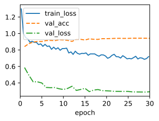
We train ConvNeXt with the compact modern recipe used in Section 7.6: AdamW, cosine decay with warmup, label smoothing, and Mixup. For a controlled local comparison, we train a ResNet-18 whose base width is reduced from 64 to 35 channels, giving it nearly the same parameter count as our ConvNeXt. The two models share the data, recipe, epoch budget, and the same seed.
TensorFlow implements the complete block, including stochastic depth, but omits this repeated comparative training run. The corresponding AdamW, warmup-cosine, label-smoothing, and Mixup components appear in Section 7.6.
The MXNet path above implements the deterministic ConvNeXt transformation but omits stochastic depth and this repeated training comparison. Its available AdamW, cosine-schedule, label-smoothing, and Mixup components are demonstrated in Section 7.6.
def cosine_warmup(epoch, max_epochs, base_lr, warmup=3):
    if epoch < warmup:
        return base_lr * (epoch + 1) / warmup
    t = (epoch - warmup) / (max_epochs - warmup)
    return base_lr * 0.5 * (1 + math.cos(math.pi * t))

def mixup(X, y, alpha):
    lam = float(torch.distributions.Beta(alpha, alpha).sample())
    perm = torch.randperm(X.shape[0], device=X.device)
    return lam * X + (1 - lam) * X[perm], y, y[perm], lam

class RecipeTrainer(d2l.Trainer):
    """A Trainer that sets the learning rate from the model's schedule."""
    def fit_epoch(self):
        for group in self.optim.param_groups:
            group['lr'] = cosine_warmup(self.epoch, self.max_epochs,
                                        self.model.lr)
        super().fit_epoch()

class ModernConvNeXt(ConvNeXt):
    """ConvNeXt under the modern recipe of the previous section."""
    def __init__(self, lr=2e-3, num_classes=10, drop_path_max=0.0):
        super().__init__(lr, num_classes, drop_path_max)

    def configure_optimizers(self):
        return torch.optim.AdamW(self.parameters(), lr=self.lr,
                                 weight_decay=0.05)

    def loss(self, y_hat, y):
        return F.cross_entropy(y_hat, y, label_smoothing=0.1)

    def training_step(self, batch):
        X, y_a, y_b, lam = mixup(*batch, alpha=0.2)
        y_hat = self(X)
        l = lam * self.loss(y_hat, y_a) + (1 - lam) * self.loss(y_hat, y_b)
        self.plot('loss', l, train=True)
        return l

class CompactResNet18(d2l.Classifier):
    """A parameter-matched ResNet-18 with base width 35."""
    def __init__(self, lr=2e-3, num_classes=10, base=35):
        super().__init__()
        self.save_hyperparameters()
        channels = (base, 2 * base, 4 * base, 8 * base)
        layers = [nn.Conv2d(1, base, 7, stride=2, padding=3),
                  nn.BatchNorm2d(base), nn.ReLU(),
                  nn.MaxPool2d(3, stride=2, padding=1)]
        for i, c in enumerate(channels):
            for j in range(2):
                down = i > 0 and j == 0
                layers.append(d2l.Residual(c, use_1x1conv=down,
                                           strides=2 if down else 1))
        layers += [nn.AdaptiveAvgPool2d((1, 1)), nn.Flatten(),
                   nn.Linear(channels[-1], num_classes)]
        self.net = nn.Sequential(*layers)

    configure_optimizers = ModernConvNeXt.configure_optimizers
    loss = ModernConvNeXt.loss
    training_step = ModernConvNeXt.training_step
def mixup(key, X, y, alpha):
key_lam, key_perm = jax.random.split(key)
lam = jax.random.beta(key_lam, alpha, alpha)
perm = jax.random.permutation(key_perm, X.shape[0])
return lam * X + (1 - lam) * X[perm], y, y[perm], lam
class ModernConvNeXt(ConvNeXt):
def __init__(self, lr=2e-3, num_classes=10, drop_path_max=0.0,
max_epochs=30, steps_per_epoch=468, rngs=None):
super().__init__(lr=lr, num_classes=num_classes,
drop_path_max=drop_path_max, rngs=rngs)
self.max_epochs, self.steps_per_epoch = max_epochs, steps_per_epoch
def configure_optimizers(self):
total = self.max_epochs * self.steps_per_epoch
schedule = optax.warmup_cosine_decay_schedule(
0.0, self.lr, 3 * self.steps_per_epoch, total)
return optax.adamw(schedule, weight_decay=0.05)
def training_step(self, batch):
X, y = batch
X, y_a, y_b, lam = mixup(self.rngs.mixup(), X, y, 0.2)
logp = jax.nn.log_softmax(self(X))
eye = jnp.eye(self.num_classes)
ta = 0.9 * eye[y_a] + 0.1 / self.num_classes
tb = 0.9 * eye[y_b] + 0.1 / self.num_classes
return (lam * -(ta * logp).sum(axis=1).mean()
+ (1 - lam) * -(tb * logp).sum(axis=1).mean())
class CompactResNet18(d2l.Classifier):
def __init__(self, lr=2e-3, num_classes=10, base=35, max_epochs=30,
steps_per_epoch=468, rngs=None):
super().__init__()
self.save_hyperparameters(ignore=['rngs'])
rngs = (nnx.Rngs(params=d2l.get_key(), dropout=d2l.get_key(),
mixup=d2l.get_key()) if rngs is None else rngs)
self.rngs = rngs
channels = (base, 2 * base, 4 * base, 8 * base)
layers = [nnx.Conv(1, base, (7, 7), strides=(2, 2),
padding='same', rngs=rngs),
nnx.BatchNorm(base, rngs=rngs), nnx.relu,
lambda x: nnx.max_pool(x, (3, 3), (2, 2), padding='SAME')]
in_channels = base
for i, c in enumerate(channels):
for j in range(2):
down = i > 0 and j == 0
layers.append(d2l.Residual(
c, use_1x1conv=down,
strides=(2, 2) if down else (1, 1),
in_channels=in_channels, rngs=rngs))
in_channels = c
layers += [lambda x: x.mean(axis=(1, 2)),
nnx.Linear(channels[-1], num_classes, rngs=rngs)]
self.net = nnx.Sequential(*layers)
configure_optimizers = ModernConvNeXt.configure_optimizers
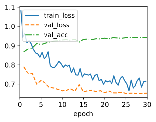
training_step = ModernConvNeXt.training_stepWe train for 30 epochs on the full Fashion-MNIST training set at \(96 \times 96\), matching the modern-recipe ResNet-18 run of Section 7.6 epoch for epoch. We set ConvNeXt’s stochastic depth rate to zero in this comparison because the compact ResNet control does not use it; the block implementation above still exercises the complete stochastic-depth path.
data = d2l.FashionMNIST(batch_size=128, resize=(96, 96))

def train_model(model_cls, seed):
    torch.manual_seed(seed)
    model = model_cls(lr=2e-3)
    trainer = RecipeTrainer(max_epochs=30, num_gpus=1)
    trainer.fit(model, data)
    model.eval()
    correct, n = 0.0, 0
    with torch.no_grad():
        for X, y in map(trainer.prepare_batch, data.val_dataloader()):
            correct += float(model.accuracy(
                model(X), y, averaged=False).sum())
            n += len(y)
    return model, correct / n

scores, models = {}, {}
for name, cls in (('ConvNeXt', ModernConvNeXt),
                  ('compact ResNet-18', CompactResNet18)):
    model, acc = train_model(cls, seed=1)
    models[name] = model
    scores[name] = acc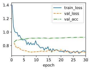
data = d2l.FashionMNIST(batch_size=128, resize=(96, 96))
jax_scores = {}
for name, model in (
        ('ConvNeXt', ModernConvNeXt(
            steps_per_epoch=len(data.train_dataloader()))),
        ('compact ResNet-18', CompactResNet18(
            steps_per_epoch=len(data.train_dataloader())))):
    d2l.tf.random.set_seed(1)  # Match the tf.data order between models
    trainer = d2l.Trainer(max_epochs=30, num_gpus=1)
    trainer.fit(model, data)
    correct, n = 0.0, 0
    for X, y in data.val_dataloader():
        values = model.accuracy(trainer.val_model(X), y, averaged=False)
        correct += float(values.sum())
        n += len(y)
    jax_scores[name] = correct / n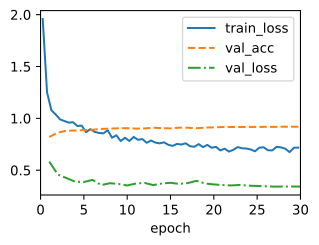
for name, acc in scores.items():
    count = sum(p.numel() for p in models[name].parameters())
    print(f'{name}: {count:,} parameters, val acc {acc:.3f}')
ConvNeXt: 3,376,450 parameters, val acc 0.923
compact ResNet-18: 3,348,320 parameters, val acc 0.944jax_scores{'ConvNeXt': 0.9183, 'compact ResNet-18': 0.9423}:The scaled-down ConvNeXt and a parameter-matched ResNet-18 under the compact modern recipe (full Fashion-MNIST at \(96 \times 96\); test accuracy, one seeded run each, rounded).
| Model | Parameters | PyTorch accuracy | JAX accuracy |
|---|---|---|---|
| ConvNeXt | 3,376,450 | ≈92% | ≈92% |
| Compact ResNet-18 | 3,348,320 | ≈94% | ≈94.5% |
This comparison asks a narrower question than the earlier run against the 11.2-million-parameter ResNet-18: at roughly 3.4 million parameters, do the ConvNeXt block and stem help on upsampled Fashion-MNIST? Each entry is one seeded run, rounded to the half point; the independent JAX run checks that the result is not tied to one implementation. Here the compact ResNet is ahead by about two points in both implementations. Even this control is task-specific: it matches parameters, not latency or multiply-adds, and every step in the published roadmap was selected on ImageNet at \(224\times224\). The local result therefore says that ConvNeXt’s ImageNet design choices do not automatically transfer to this small grayscale task; it is not a general ranking of the architecture families.
7.7.3 Beyond ConvNeXt
7.7.3.1 ConvNeXt V2: pretraining and GRN
ConvNeXt closed the supervised gap, but by 2023 the frontier had moved to self-supervised pretraining, where transformers held an advantage: masked autoencoders (He et al. 2022) drop most input patches and train the network to reconstruct them, which is natural for a patch-sequence model and awkward for a convolution that slides across the holes. ConvNeXt V2 (Woo et al. 2023) adapted the idea with sparse convolutions that skip masked regions during pretraining. Doing so exposed a failure the authors traced to feature collapse: with the V1 block, many channels of the pretrained network become inactive or redundant. Their proposed remedy is Global Response Normalization (GRN), a three-line layer inserted after the block’s GELU: it computes each channel’s global response norm, divides by the mean over channels, and uses the ratio to recalibrate the features, sharpening the contrast between channels and preventing collapse. It also replaces layer scale. The combination of the masked-autoencoder pretraining and GRN lifted the largest model to 88.9% ImageNet top-1 accuracy, which the authors reported as the strongest result then trained on public data. Implementing GRN is one of the exercises, and it fits in about five lines.
7.7.3.2 Large Kernels and Other Spatial Mixers
The roadmap’s \(7 \times 7\) kernel motivates testing still larger kernels. RepLKNet (Ding et al. 2022) pushed depthwise kernels to \(31 \times 31\), using the re-parameterization method of Section 7.5 to train a parallel small kernel that folds away at inference, and showed the effective receptive field widening dramatically, with the gains showing up mostly in detection and segmentation rather than classification. SLaK (S. Liu et al. 2022) reached \(51 \times 51\) by factorizing the kernel into two thin rectangular stripes plus dynamic sparsity. InternImage (Wang et al. 2023) took the opposite route to the same goal, a large adaptive receptive field, by building its blocks from deformable convolutions (DCNv3) whose sampling locations are input-dependent, and scaled to 3 billion parameters and state-of-the-art COCO detection. UniRepLKNet (Ding et al. 2024) carried large-kernel design across modalities, to audio, point clouds, and time series.
The durable result is narrower than a verdict on one winning operator. Modern backbones need access to wide context, and ConvNeXt showed that a moderately large depthwise kernel is one practical way to obtain it. Fixed kernels of \(31 \times 31\) and beyond have remained specialized: their reported gains are strongest in dense prediction, and efficient training or inference often needs re-parameterization, sparsity, or specialized kernels. Deformable operators and attention provide alternative, input-dependent routes to wide context.
7.7.3.3 ConvNeXt in 2026
ConvNeXt has aged into infrastructure. It is a standard strong-CNN backbone in detection and segmentation toolkits, a common encoder choice where a transformer’s quadratic attention cost is unwelcome at high resolution, and the convolutional tower in several widely used OpenCLIP image-text models (Radford et al. 2021), where ConvNeXt encoders trained on billion-scale image-text corpora remain among the strongest public convolutional models. When a practitioner chooses a CNN, the CNN they reach for is more often than not a ConvNeXt or something shaped like one.
7.7.4 Summary and Discussion
ConvNeXt is a controlled experiment wearing an architecture’s name. One change at a time, it turned a 2015 ResNet-50 into a network that matches Swin at equal cost: a modern recipe, a Swin-like stage ratio, a patchify stem, depthwise convolutions in an inverted bottleneck led by a \(7 \times 7\) kernel, GELU, and fewer normalization and activation layers. At the scales tested in the paper, well-tuned convnets and transformers are competitive; the experiment does not establish that either family dominates in every data and compute regime. Our parameter-matched Fashion-MNIST comparison applies the same control discipline to the smaller setting used in this book.
The block itself is a piece of convergent evolution. A depthwise convolution that mixes space but not channels, a pointwise MLP that expands by four and mixes channels but not space, one normalization, one activation, a residual connection: strip the names and the ConvNeXt block and the transformer block are the same design with different spatial mixers. That reading, which Section 7.8 develops, is more durable than any single leaderboard number, including the ones in this section.
7.7.5 Exercises
The training comparison of Table 7.7.2 runs in PyTorch and JAX. To work the training problems below in Keras, build its ResNet-18 control from the ResNet of Section 7.4 with arch=((2, 35), (2, 70), (2, 140), (2, 280)) and the stem narrowed from 64 to 35 channels, and reuse the AdamW optimizer with the CosineDecay schedule, CategoricalCrossentropy with label_smoothing, and mixup of Section 7.6.
The training comparison of Table 7.7.2 runs in PyTorch and JAX. To work the training problems below in Gluon, build its ResNet-18 control from the ResNet of Section 7.4 with arch=((2, 35), (2, 70), (2, 140), (2, 280)) and the stem narrowed from 64 to 35 channels, and reuse the AdamW optimizer, CosineScheduler, smoothed_ce, and mixup of Section 7.6.
- Roadmap ablations. The roadmap in Table 7.7.1 applies its changes in one fixed order, and each row’s gain is measured with every earlier change in place.
- Just before the “Large kernels” row, each block expands its residual width \(c\) to \(4c\) with a \(1 \times 1\) convolution, applies a \(3 \times 3\) depthwise convolution to the \(4c\) channels, and projects back to \(c\) with a second \(1 \times 1\) convolution. The row first moves the depthwise convolution in front of the expansion, where it acts on \(c\) channels, and then enlarges its kernel to \(7 \times 7\). Count the multiply-adds per spatial position of the depthwise convolution before the move, after the move, and after the enlargement. Compare the net change over the row with the change that enlarging the kernel to \(7 \times 7\) in place, on the \(4c\) channels, would have caused.
- Choose two rows whose gains you expect to depend on their order, and design the additional runs that would measure the interaction.
- Where the parameters live.
- For the
ConvNeXtof this section, compute the fraction of parameters in the depthwise convolutions, in the \(1 \times 1\) expansions and projections, in the normalizations and layer-scale vectors inside the blocks, in the downsampling layers, and in the stem and head. Check that the total is 3,376,450. - Express the parameter count of a
ConvNeXtBlockand of aResidualblock of Section 7.4 without the \(1 \times 1\) shortcut as functions of the width \(c\). Which design decision makes the ConvNeXt block cheaper, and by what factor for large \(c\)?
- For the
- Normalization axes. The activations entering a normalization layer form a minibatch of \(n\) images, each with \(c\) channels on an \(h \times w\) map. Consider three layers: batch normalization, the per-position layer normalization of
ConvNeXtBlock, and a layer normalization over all \(chw\) values of an image with one learnable scale and one learnable shift per value.- For each layer, state which values share one mean and variance, and count its learnable parameters.
- A network trained on \(96 \times 96\) images is evaluated on \(224 \times 224\) images. Which of the three layers can be applied to the larger images with their trained parameters unchanged? Explain.
- [code] Depthwise kernel size. ● Under the compact modern recipe of Table 7.7.2, train
ConvNeXtwith \(3 \times 3\) and with \(11 \times 11\) depthwise convolutions that leave the feature-map size unchanged, and compare accuracy, parameter count, and time per epoch against the \(7 \times 7\) baseline. Does accuracy saturate at \(7 \times 7\) here as Z. Liu et al. (2022) report on ImageNet? How does the change in time per epoch compare with the change in the depthwise term’s arithmetic, and why? - [code] Layer scale. Under the compact modern recipe of Table 7.7.2, train
ConvNeXtwith \(\gamma\) initialized to \(10^{-6}\) (the default), with \(\gamma\) initialized to \(1\), and with layer scale removed, and compare the training curves. Layer scale at \(10^{-6}\) and stochastic depth (Equation 7.6.4) both make the network effectively shallower than its block count. For each mechanism, explain how it does so, state when during training it acts, and state whether it changes the network used at evaluation. - [code] Global Response Normalization. ConvNeXt V2 (Woo et al. 2023) inserts GRN after the GELU of the block and removes layer scale. For a feature map \(\mathbf{X}\) with \(C\) channels, let \(g_c\) be the \(\ell_2\) norm of channel \(c\) over all spatial positions and \(\bar{g}\) the mean of \(g_1, \ldots, g_C\). GRN rescales each channel by its normalized response and adds a learnable per-channel affine term and a residual, \[\mathrm{GRN}(\mathbf{X})_c = \gamma_c \frac{g_c}{\bar{g}} \mathbf{X}_c + \beta_c + \mathbf{X}_c, \tag{7.7.1}\] with \(\gamma_c\) and \(\beta_c\) initialized to zero so that the layer starts as the identity.
- Implement GRN in about five lines and insert it into
ConvNeXtBlockafter the GELU, dropping layer scale. - Retrain under the compact modern recipe and compare the test accuracy with Table 7.7.2.
- Implement GRN in about five lines and insert it into
- [code] Channel redundancy. ● Take the
ConvNeXttrained with GRN in the previous problem and the one trained without it under the same recipe. Measure the channel redundancy that GRN was designed to prevent, at the input of the second \(1 \times 1\) convolution of every block. For each test image, flatten each channel’s map into a vector over the spatial positions, and average the cosine similarity over all pairs of channels. Average over the test images and compare the networks with and without GRN block by block. In which stages, if any, does GRN make the channels less similar? - [code] Recipe downgrade. ● The comparison in Table 7.7.2 trains two architectures under the compact modern recipe. Complete the ablation square by training both models under recipe A of Section 7.6: SGD with momentum, step decay, and neither Mixup nor label smoothing, with the learning rate retuned. How much of each network’s accuracy survives the downgrade, and does the recipe help both architectures equally? Compare the size of the effect with the 2.7 points that the “Modern training recipe” row of Table 7.7.1 attributes to the recipe on ImageNet.