from d2l import torch as d2l
import torch
from torch import nn
import random23.6 Neural Collaborative Filtering for Personalized Ranking
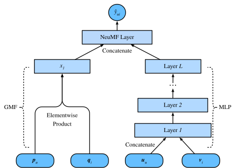
Clicks, purchases, and viewing events are easier to record than explicit ratings, but they pose a different statistical problem. An observed event is evidence of interest; an unobserved event may instead reflect a lack of exposure. We therefore seek a score that ranks plausible items for each user, and train it against sampled unobserved items. Neural matrix factorization (NeuMF) (He et al. 2017) constructs this score from two complementary feature maps: an elementwise interaction, closely related to matrix factorization, and a multilayer network applied to the user and item embeddings.
23.6.1 The NeuMF model
The generalized matrix factorization (GMF) branch associates user \(u\) and item \(i\) with vectors \(\mathbf{p}_u,\mathbf{q}_i\in\mathbb{R}^k\) and forms
\[ \begin{aligned} \mathbf{x}_{\mathrm{GMF}} = \mathbf{p}_u \odot \mathbf{q}_i, \end{aligned} \]
where \(\odot\) denotes elementwise multiplication. Unlike the dot product \(\mathbf{p}_u^\top\mathbf{q}_i\), this operation retains all \(k\) coordinatewise products for the final prediction layer.
The multilayer perceptron (MLP) branch uses separate embeddings \(\mathbf{U}_u\) and \(\mathbf{V}_i\). Starting from their concatenation, it computes
\[ \begin{aligned} \mathbf{z}^{(1)} &= [\mathbf{U}_u;\mathbf{V}_i], \\ \mathbf{z}^{(\ell)} &= \alpha_\ell\!\left(\mathbf{W}^{(\ell)}\mathbf{z}^{(\ell-1)}+\mathbf{b}^{(\ell)}\right), \qquad \ell=2,\ldots,L, \end{aligned} \]
where \([\cdot;\cdot]\) denotes concatenation and \(\alpha_\ell\) is the activation at layer \(\ell\). Separate embeddings allow the two branches to represent users and items in coordinate systems suited to their respective computations.
NeuMF concatenates the two feature vectors and applies a learned linear readout. Because BPR depends only on score differences, the implementation returns the raw score \[ s_{ui} = \mathbf{h}^\top[\mathbf{x}_{\mathrm{GMF}};\mathbf{z}^{(L)}]. \] A sigmoid may convert this logit to a pointwise probability in a separately calibrated model, but it should not be inserted before the BPR score difference.
from d2l import mxnet as d2l
from mxnet import autograd, gluon, np, npx
from mxnet.gluon import nn
import mxnet as mx
import random

npx.set_np()
23.6.2 Model Implementation
The following code implements the NeuMF model. It consists of a generalized matrix factorization model and an MLP with different user and item embedding vectors. The structure of the MLP is controlled with the parameter nums_hiddens. ReLU is used as the default activation function.
class NeuMF(nn.Module):
    def __init__(self, num_factors, num_users, num_items, nums_hiddens):
        super().__init__()
        self.P = nn.Embedding(num_users, num_factors)
        self.Q = nn.Embedding(num_items, num_factors)
        self.U = nn.Embedding(num_users, num_factors)
        self.V = nn.Embedding(num_items, num_factors)
        mlp_layers = []
        input_size = num_factors * 2
        for num_hiddens in nums_hiddens:
            mlp_layers.append(nn.Linear(input_size, num_hiddens))
            mlp_layers.append(nn.ReLU())
            input_size = num_hiddens
        self.mlp = nn.Sequential(*mlp_layers)
        # Output raw logits; BPRLoss applies sigmoid internally, so adding
        # a sigmoid here would compose with it and squash gradients.
        self.prediction_layer = nn.Linear(num_factors + nums_hiddens[-1], 1,
                                          bias=False)

    def forward(self, user_id, item_id):
        p_mf = self.P(user_id)
        q_mf = self.Q(item_id)
        gmf = p_mf * q_mf
        p_mlp = self.U(user_id)
        q_mlp = self.V(item_id)
        mlp = self.mlp(torch.cat([p_mlp, q_mlp], dim=1))
        con_res = torch.cat([gmf, mlp], dim=1)
        return self.prediction_layer(con_res)
class NeuMF(nn.Block):
def __init__(self, num_factors, num_users, num_items, nums_hiddens):
super().__init__()
self.P = nn.Embedding(num_users, num_factors)
self.Q = nn.Embedding(num_items, num_factors)
self.U = nn.Embedding(num_users, num_factors)
self.V = nn.Embedding(num_items, num_factors)
self.mlp = nn.Sequential()
for num_hiddens in nums_hiddens:
self.mlp.add(nn.Dense(num_hiddens, activation='relu',
use_bias=True))
# Output raw logits; BPRLoss applies sigmoid internally, so adding
# a sigmoid here would compose with it and squash gradients.
self.prediction_layer = nn.Dense(1, use_bias=False)
def forward(self, user_id, item_id):
p_mf = self.P(user_id)
q_mf = self.Q(item_id)
gmf = p_mf * q_mf
p_mlp = self.U(user_id)
q_mlp = self.V(item_id)
mlp = self.mlp(np.concatenate([p_mlp, q_mlp], axis=1))
con_res = np.concatenate([gmf, mlp], axis=1)
return self.prediction_layer(con_res)23.6.3 Customized Dataset with Negative Sampling
For pairwise ranking, the sampling distribution is part of the objective. The following dataset samples uniformly from the complement of each user’s observed training items. Samples are redrawn on every access, so repeated epochs compare an observed item with different unobserved items.
This compact experiment also removes the held-out positive from the sampling pool. That avoids assigning opposite labels to the same item, but it consults the identity of the evaluation event during training. A strict final test would instead tune this choice on validation users or define a proposal without using test labels, then reserve test identities until evaluation.
class PRDataset(torch.utils.data.Dataset):
    def __init__(self, users, items, candidates, num_items, test_items=None):
        self.users = users
        self.items = items
        # Precompute each user's negative pool once: items the user has not
        # interacted with in train, excluding the known held-out positive.
        # This avoids a contradictory sampled label but uses evaluation identity;
        # see the protocol limitation in the surrounding text.
        all_items = set(range(num_items))
        test_items = test_items or {}
        self.neg_pool = {
            u: list(all_items - set(candidates.get(u, [])) - set(test_items.get(u, [])))
            for u in candidates}

    def __len__(self):
        return len(self.users)

    def __getitem__(self, idx):
        neg_items = self.neg_pool[int(self.users[idx])]
        indices = random.randint(0, len(neg_items) - 1)
        return self.users[idx], self.items[idx], neg_items[indices]
class PRDataset(gluon.data.Dataset):
def __init__(self, users, items, candidates, num_items, test_items=None):
self.users = users
self.items = items
# Precompute each user's negative pool once: items the user has not
# interacted with in train, excluding the known held-out positive.
# This avoids a contradictory sampled label but uses evaluation identity;
# see the protocol limitation in the surrounding text.
all_items = set(range(num_items))
test_items = test_items or {}
self.neg_pool = {
u: list(all_items - set(candidates.get(u, [])) - set(test_items.get(u, [])))
for u in candidates}
def __len__(self):
return len(self.users)
def __getitem__(self, idx):
neg_items = self.neg_pool[int(self.users[idx])]
indices = random.randint(0, len(neg_items) - 1)
return self.users[idx], self.items[idx], neg_items[indices]23.6.4 Evaluation on a Chronological Holdout
For each user \(u\), the final observed item \(g_u\) is held out and ranked within an evaluation candidate set \(C_u\) that contains \(g_u\) and items not observed in the training history. The candidate set is part of the protocol: ranking against every item and ranking against a sampled subset generally produce different values. The hit rate at cutoff \(\ell\) is
\[ \operatorname{Hit}@\ell = \frac{1}{|\mathcal{U}|}\sum_{u\in\mathcal{U}}\mathbf{1}\{\operatorname{rank}_u(g_u)\leq\ell\}. \]
It records whether the held-out item appears among the first \(\ell\) candidates, then averages over users. The corresponding per-user AUC is the fraction of other candidates scored below the held-out item:
\[ \operatorname{AUC}=\frac{1}{|\mathcal{U}|}\sum_{u\in\mathcal{U}}\frac{1}{|C_u|-1}\sum_{j\in C_u\setminus\{g_u\}}\mathbf{1}\{\hat y_{u g_u}>\hat y_{uj}\}. \]
The formula assigns no credit to ties; a protocol that awards half credit must say so explicitly. Hit rate and AUC answer different questions, and neither corrects for the fact that a held-out click reflects both exposure and preference.
The following function calculates the hit counts and AUC for each user.
def hit_and_auc(rankedlist, test_matrix, k):
    hits_k = [(idx, val) for idx, val in enumerate(rankedlist[:k])
              if val in set(test_matrix)]
    hits_all = [(idx, val) for idx, val in enumerate(rankedlist)
                if val in set(test_matrix)]
    max = len(rankedlist) - 1
    auc = 1.0 * (max - hits_all[0][0]) / max if len(hits_all) > 0 else 0
    return len(hits_k), auc
def hit_and_auc(rankedlist, test_matrix, k):
    hits_k = [(idx, val) for idx, val in enumerate(rankedlist[:k])
              if val in set(test_matrix)]
    hits_all = [(idx, val) for idx, val in enumerate(rankedlist)
                if val in set(test_matrix)]
    max = len(rankedlist) - 1
    auc = 1.0 * (max - hits_all[0][0]) / max if len(hits_all) > 0 else 0
    return len(hits_k), auc
Then, the overall Hit rate and AUC are calculated as follows. Note that evaluate_ranking rebuilds and sorted-ranks each user’s candidate scores in a per-user Python loop for clarity; the efficient form would score all users in a batch and select the top items with a single top-k call (PyTorch’s torch.topk).
def evaluate_ranking(net, test_input, seq, candidates, num_users, num_items,
                     devices):
    ranked_list, ranked_items, hit_rate, auc = {}, {}, [], []
    all_items = set([i for i in range(num_items)])
    for u in range(num_users):
        neg_items = list(all_items - set(candidates[int(u)]))
        user_ids, item_ids, scores = [], [], []
        [item_ids.append(i) for i in neg_items]
        [user_ids.append(u) for _ in neg_items]
        x = [torch.tensor(user_ids)]
        if seq is not None:
            x.append(seq[user_ids, :])
        x.extend([torch.tensor(item_ids)])
        test_data_iter = torch.utils.data.DataLoader(
            torch.utils.data.TensorDataset(*x), shuffle=False,
            batch_size=1024)
        for values in test_data_iter:
            values = [v.to(devices[0]) for v in values]
            # `net` returns a 1-D tensor of logits per batch; ravel
            # ensures we always extend with scalars regardless of whether
            # the model emits shape (B,) or (B, 1).
            scores.extend(net(*values).detach().cpu().numpy().ravel().tolist())
        item_scores = list(zip(item_ids, scores))
        ranked_list[u] = sorted(item_scores, key=lambda t: t[1], reverse=True)
        ranked_items[u] = [r[0] for r in ranked_list[u]]
        temp = hit_and_auc(ranked_items[u], test_input[u], 50)
        hit_rate.append(temp[0])
        auc.append(temp[1])
    return sum(hit_rate) / len(hit_rate), sum(auc) / len(auc)
def evaluate_ranking(net, test_input, seq, candidates, num_users, num_items,
                     devices):
    ranked_list, ranked_items, hit_rate, auc = {}, {}, [], []
    all_items = set([i for i in range(num_items)])
    for u in range(num_users):
        neg_items = list(all_items - set(candidates[int(u)]))
        user_ids, item_ids, x, scores = [], [], [], []
        [item_ids.append(i) for i in neg_items]
        [user_ids.append(u) for _ in neg_items]
        x.extend([np.array(user_ids)])
        if seq is not None:
            x.append(seq[user_ids, :])
        x.extend([np.array(item_ids)])
        test_data_iter = gluon.data.DataLoader(
            gluon.data.ArrayDataset(*x), shuffle=False, last_batch="keep",
            batch_size=1024)
        for index, values in enumerate(test_data_iter):
            x = [gluon.utils.split_and_load(v, devices, even_split=False)
                 for v in values]
            scores.extend([list(net(*t).asnumpy()) for t in zip(*x)])
        scores = [item for sublist in scores for item in sublist]
        item_scores = list(zip(item_ids, scores))
        ranked_list[u] = sorted(item_scores, key=lambda t: t[1], reverse=True)
        ranked_items[u] = [r[0] for r in ranked_list[u]]
        temp = hit_and_auc(ranked_items[u], test_input[u], 50)
        hit_rate.append(temp[0])
        auc.append(temp[1])
    return np.mean(np.array(hit_rate)), np.mean(np.array(auc))
23.6.5 Training and Evaluating the Model
The training function is defined below. We train the model in the pairwise manner.
def train_ranking(net, train_iter, test_iter, loss, optimizer, test_seq_iter,
                  num_users, num_items, num_epochs, devices, evaluator,
                  candidates, eval_step=1):
    timer, hit_rate, auc = d2l.Timer(), 0, 0
    animator = d2l.Animator(xlabel='epoch', xlim=[1, num_epochs], ylim=[0, 1],
                            legend=['test hit rate', 'test AUC'])
    for epoch in range(num_epochs):
        metric = d2l.Accumulator(3)
        for i, values in enumerate(train_iter):
            input_data = [v.to(devices[0]) for v in values]
            p_pos = net(*input_data[:-1])
            p_neg = net(*input_data[:-2], input_data[-1])
            ls = loss(p_pos, p_neg)
            optimizer.zero_grad()
            ls.backward()
            optimizer.step()
            # Per-batch loss only; accumulating across batches inside `l`
            # turned the printed train-loss into a quadratic sum.
            metric.add(ls.item(), values[0].shape[0], values[0].numel())
            timer.stop()
        with torch.no_grad():
            if (epoch + 1) % eval_step == 0:
                hit_rate, auc = evaluator(net, test_iter, test_seq_iter,
                                          candidates, num_users, num_items,
                                          devices)
                animator.add(epoch + 1, (hit_rate, auc))
    print(f'train loss {metric[0] / metric[1]:.3f}, '
          f'test hit rate {float(hit_rate):.3f}, test AUC {float(auc):.3f}')
    print(f'{metric[2] * num_epochs / timer.sum():.1f} examples/sec '
          f'on {str(devices)}')
def train_ranking(net, train_iter, test_iter, loss, trainer, test_seq_iter,
                  num_users, num_items, num_epochs, devices, evaluator,
                  candidates, eval_step=1):
    timer, hit_rate, auc = d2l.Timer(), 0, 0
    animator = d2l.Animator(xlabel='epoch', xlim=[1, num_epochs], ylim=[0, 1],
                            legend=['test hit rate', 'test AUC'])
    for epoch in range(num_epochs):
        metric = d2l.Accumulator(3)
        for i, values in enumerate(train_iter):
            input_data = []
            for v in values:
                input_data.append(gluon.utils.split_and_load(v, devices))
            with autograd.record():
                p_pos = [net(*t) for t in zip(*input_data[:-1])]
                p_neg = [net(*t) for t in zip(*input_data[:-2],
                                              input_data[-1])]
                ls = [loss(p, n) for p, n in zip(p_pos, p_neg)]
            [l.backward(retain_graph=False) for l in ls]
            # Per-batch loss only; accumulating across batches inside `l`
            # turned the printed train-loss into a quadratic sum.
            batch_loss = sum([l.asnumpy() for l in ls]).mean()
            trainer.step(values[0].shape[0])
            metric.add(batch_loss, values[0].shape[0], values[0].size)
            timer.stop()
        with autograd.predict_mode():
            if (epoch + 1) % eval_step == 0:
                hit_rate, auc = evaluator(net, test_iter, test_seq_iter,
                                          candidates, num_users, num_items,
                                          devices)
                animator.add(epoch + 1, (hit_rate, auc))
    print(f'train loss {metric[0] / metric[1]:.3f}, '
          f'test hit rate {float(hit_rate):.3f}, test AUC {float(auc):.3f}')
    print(f'{metric[2] * num_epochs / timer.sum():.1f} examples/sec '
          f'on {str(devices)}')
Now, we can load the MovieLens 100k dataset and train the model. Since there are only ratings in the MovieLens dataset, with some losses of accuracy, we binarize these ratings to zeros and ones. If a user rated an item, we consider the implicit feedback as one, otherwise as zero. The action of rating an item can be treated as a form of providing implicit feedback. Here, we split the dataset in the seq-aware mode where users’ latest interacted items are left out for test.
batch_size = 1024
df, num_users, num_items = d2l.read_data_ml100k()
train_data, test_data = d2l.split_data_ml100k(df, num_users, num_items,
                                              'seq-aware')
users_train, items_train, ratings_train, candidates = d2l.load_data_ml100k(
    train_data, num_users, num_items, feedback="implicit")
users_test, items_test, ratings_test, test_iter = d2l.load_data_ml100k(
    test_data, num_users, num_items, feedback="implicit")
train_iter = torch.utils.data.DataLoader(
    PRDataset(users_train, items_train, candidates, num_items,
              test_items=test_iter), batch_size,
    True, num_workers=d2l.get_dataloader_workers())
batch_size = 1024
df, num_users, num_items = d2l.read_data_ml100k()
train_data, test_data = d2l.split_data_ml100k(df, num_users, num_items,
'seq-aware')
users_train, items_train, ratings_train, candidates = d2l.load_data_ml100k(
train_data, num_users, num_items, feedback="implicit")
users_test, items_test, ratings_test, test_iter = d2l.load_data_ml100k(
test_data, num_users, num_items, feedback="implicit")
train_iter = gluon.data.DataLoader(
PRDataset(users_train, items_train, candidates, num_items,
test_items=test_iter), batch_size,
True, last_batch="rollover", num_workers=d2l.get_dataloader_workers())We then create and initialize the model. We use a three-layer MLP with constant hidden size 10.
devices = d2l.try_all_gpus()
net = NeuMF(10, num_users, num_items, nums_hiddens=[10, 10, 10])
def init_weights(m):
    if type(m) == nn.Linear or type(m) == nn.Embedding:
        nn.init.normal_(m.weight, std=0.01)
net.apply(init_weights)
net = net.to(devices[0])
devices = d2l.try_all_gpus()
net = NeuMF(10, num_users, num_items, nums_hiddens=[10, 10, 10])
# Xavier gives the GMF and MLP branches comparable initial activation scales.
# The model returns raw scores; BPR applies a sigmoid to their difference.
net.initialize(ctx=devices, force_reinit=True, init=mx.init.Xavier())The following code trains the model.
lr, num_epochs, wd = 0.01, 10, 1e-5
loss = d2l.BPRLoss()
optimizer = torch.optim.Adam(net.parameters(), lr=lr, weight_decay=wd)
train_ranking(net, train_iter, test_iter, loss, optimizer, None, num_users,
              num_items, num_epochs, devices, evaluate_ranking, candidates)
train loss 0.152, test hit rate 0.352, test AUC 0.883
10.6 examples/sec on [device(type='cuda', index=0)]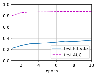
lr, num_epochs, wd, optimizer = 0.01, 10, 1e-5, 'adam'
loss = d2l.BPRLoss()
trainer = gluon.Trainer(net.collect_params(), optimizer,
                        {"learning_rate": lr, 'wd': wd})
train_ranking(net, train_iter, test_iter, loss, trainer, None, num_users,
              num_items, num_epochs, devices, evaluate_ranking, candidates,
              eval_step=5)
train loss 0.151, test hit rate 0.359, test AUC 0.881
12.9 examples/sec on [gpu(0)]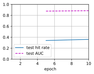
23.6.6 Summary
- NeuMF combines coordinatewise latent-factor interactions with nonlinear features computed from concatenated user and item embeddings.
- The two branches use separate embeddings and are joined only at the prediction layer.
23.6.7 Exercises
- Vary the size of latent factors. How does the size of latent factors impact the model performance?
- Vary the architectures (e.g., number of layers, number of neurons of each layer) of the MLP to check its impact on the performance.
- Try different optimizers, learning rate and weight decay rate.
- Try to use hinge loss defined in the last section to optimize this model.