%matplotlib inline
from d2l import torch as d2l
import torch
from torch.nn import functional as F
import numpy as np26.5 Numerical Stability and Conditioning
The preceding results assume exact arithmetic over the real numbers, whereas computers use finite-precision floating-point numbers. Overflow, underflow, and catastrophic cancellation can therefore invalidate a mathematically correct algorithm. This section develops stable formulations of softmax, cross-entropy, and least squares using maximum subtraction, log-space arithmetic, and ridge regularization. Numerical analysis separates error due to the algorithm from sensitivity inherent in the problem (Higham 2002). The condition number \(\kappa = \sigma_{\max}/\sigma_{\min}\) quantifies that sensitivity and also governs the convergence rate of gradient descent in Section 26.1. The same stable computations appear in naive Bayes (Section 27.7) and information-theoretic losses (Section 28.1).
We proceed in four steps: the representation and range of floating-point numbers; stable computation of softmax, log-sum-exp, and cross-entropy; why subtracting nearly equal numbers destroys digits and how reformulation (not higher precision) reduces the error; and finally conditioning: backward versus forward error, the Hilbert matrix, why normal equations square the condition number, and how ridge regularization conditions the problem the way a preconditioner does. The standard references are Goldberg (1991) for floating point and Higham (2002) for the numerical error analysis; Goodfellow et al. (2016) (chapter 4) gives the deep-learning framing. Most code in this section is plain NumPy, since these phenomena belong to the arithmetic rather than to any library; the exception is the cross-entropy experiment, where library behavior genuinely differs.
%matplotlib inline
from d2l import tensorflow as d2l
import tensorflow as tf
import ml_dtypes
import numpy as np%matplotlib inline
from d2l import jax as d2l
import jax
from jax import numpy as jnp
import optax
import numpy as np%matplotlib inline
from d2l import mxnet as d2l
from mxnet import np as mxnp, npx
npx.set_np()
import numpy as np26.5.1 Floating-Point Arithmetic
26.5.1.1 Representation and Spacing
A floating-point number is scientific notation in base \(2\) with a fixed budget of digits:
\[ x = (-1)^s \cdot (1.m_1 m_2 \ldots m_p)_2 \cdot 2^{e}, \tag{26.5.1}\]
a sign bit \(s\), a mantissa (significand) with \(p\) stored bits, and an integer exponent \(e\) from a fixed range. The exponent gives enormous range, the mantissa gives fixed relative precision, and between consecutive powers of two the representable values are evenly spaced, so the spacing doubles every time the magnitude does. Figure 26.5.1 shows the resulting number line: representable values crowd near zero and thin out toward the overflow threshold, while the relative gap between neighbors stays essentially constant.
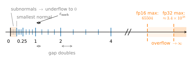
That constant relative gap has a name. Machine epsilon \(\varepsilon_{\text{mach}}\) is the distance from \(1\) to the next representable number, \(\varepsilon_{\text{mach}} = 2^{-p}\) for a \(p\)-bit mantissa. For a nonzero real \(x\) whose rounded value is finite and normal, round-to-nearest obeys
\[ \mathrm{fl}(x) = x\,(1 + \delta), \qquad |\delta| \le u = \tfrac12\,\varepsilon_{\text{mach}}, \tag{26.5.2}\]
For a correctly rounded basic operation whose exact finite result lies in the normal range, IEEE arithmetic gives the analogous model: the computed \(x \oplus y\) equals \((x + y)(1 + \delta)\) with \(|\delta| \le u\) ((IEEE 2019; Goldberg 1991)). Overflow, division by zero, NaNs, and results in the subnormal/underflow region require separate absolute-error reasoning; those exceptions are central rather than incidental below. The quantity \(u\) is the unit roundoff. Repeated operations accumulate these rounding terms, and subtraction can amplify error already present in its operands, as discussed in Section 26.5.3).
Deep-learning systems commonly use three formats. The following table obtains their parameters directly from the library:
import numpy as onp
header = f'{"dtype":>10} {"eps":>12} {"smallest normal":>17} {"max":>12}'
print(header)
for dt in [onp.float16, onp.float32]:
    fi = onp.finfo(dt)
    print(f'{onp.dtype(dt).name:>10} {fi.eps:12.3e} '
          f'{fi.smallest_normal:17.3e} {fi.max:12.3e}')

def to_bf16(x):
    """Round float32 to the nearest bfloat16 (round half to even)."""
    bits = onp.atleast_1d(onp.asarray(x, onp.float32)).view(onp.uint32)
    bits = (bits + 0x7FFF + ((bits >> 16) & 1)) & 0xFFFF0000
    return bits.astype(onp.uint32).view(onp.float32)

eps_bf16 = (to_bf16(1.0 + 2.0**-7) - 1.0).item()  # emulated: mxnet has no bf16
print(f'{"bfloat16":>10} {eps_bf16:12.3e}   (exponent range = float32)')
print('bfloat16 eps equals 2^-7:', eps_bf16 == 2.0**-7,
      ' and 1 + 2^-8 rounds back to 1:', to_bf16(1.0 + 2.0**-8).item() == 1.0)
dtype eps smallest normal max
float16 9.766e-04 6.104e-05 6.550e+04
float32 1.192e-07 1.175e-38 3.403e+38
bfloat16 7.812e-03 (exponent range = float32)
bfloat16 eps equals 2^-7: True and 1 + 2^-8 rounds back to 1: TrueThe three formats make different precision–range tradeoffs. fp32 (\(p = 23\) mantissa bits) has \(\varepsilon_{\text{mach}} = 2^{-23} \approx 1.19 \times 10^{-7}\), about seven decimal digits, with range up to \(3.4 \times 10^{38}\). fp16 (\(p = 10\)) keeps \(\varepsilon_{\text{mach}} = 2^{-10} \approx 9.8 \times 10^{-4}\) but has a small exponent range: it overflows at \(65504\) and its smallest normal number is about \(6.1 \times 10^{-5}\), so big activations overflow and small gradients underflow. bfloat16 (\(p = 7\)) makes the opposite trade: it keeps fp32’s full exponent range and sacrifices the mantissa, leaving \(\varepsilon_{\text{mach}} = 2^{-7} = 0.0078\), between two and three decimal digits. The printout confirms the value that is easy to misquote: bfloat16’s epsilon is \(2^{-7}\), not \(2^{-8}\); the eighth mantissa bit people sometimes count is the implicit leading \(1\) in Equation 26.5.1, which fills no gap.
Since 2022, hardware has extended this progression to fp8, standardized in two formats (Micikevicius et al. 2022). E4M3 (\(p=3\)) has \(\varepsilon_{\text{mach}}=2^{-3}=0.125\), roughly one decimal digit of precision, and a maximum magnitude of \(448\). E5M2 (\(p=2\)) gives up one mantissa bit in exchange for fp16’s exponent range, with maximum \(57344\) and smallest normal value \(6.1\times10^{-5}\). E4M3 is often used for weights and activations, where precision is important, while E5M2 is useful for gradients that require greater range. Practical fp8 training uses tensor- or block-level scale factors to keep values inside the representable interval. The reduced bit budget therefore trades precision and range against scaling overhead.
for dt in [torch.float8_e4m3fn, torch.float8_e5m2]:
    fi = torch.finfo(dt)
    print(f'{str(dt)[6:]:>13}  eps = {fi.eps:5}  '
          f'smallest normal = {fi.smallest_normal:12}  max = {fi.max:7}')
float8_e4m3fn eps = 0.125 smallest normal = 0.015625 max = 448.0
float8_e5m2 eps = 0.25 smallest normal = 6.103515625e-05 max = 57344.0The printout shows the tradeoff directly. With three mantissa bits, E4M3 has epsilon \(0.125\) and maximum \(448\). E5M2 uses two mantissa bits, so its epsilon is \(0.25\), but its maximum is \(57344\) and its smallest normal value is \(6.1\times10^{-5}\), matching fp16’s exponent range.
The following experiments illustrate \(\varepsilon_{\text{mach}}\). Adding half an epsilon to \(1\) rounds back to \(1\), and the absolute gap between adjacent values is about a million times larger at \(2^{20}\) than at \(1\):
eps = np.finfo(np.float32).eps
one = np.float32(1.0)
print('1 + eps   != 1 :', one + eps != one)
print('1 + eps/2 == 1 :', one + np.float32(eps / 2) == one)
print('gap between adjacent float32 values near 1    :',
      np.spacing(np.float32(1.0)))
print('gap between adjacent float32 values near 2^20 :',
      np.spacing(np.float32(2.0**20)))
for dt in [np.float16, np.float32]:
    print(f'{np.dtype(dt).name}: exp(x) overflows for x >',
          f'{np.log(np.finfo(dt).max):.2f}')
1 + eps != 1 : True
1 + eps/2 == 1 : True
gap between adjacent float32 values near 1 : 1.1920929e-07
gap between adjacent float32 values near 2^20 : 0.125
float16: exp(x) overflows for x > 11.09
float32: exp(x) overflows for x > 88.7226.5.1.2 Overflow, Underflow, and Mixed Precision
The last two printed lines locate the thresholds that matter most in practice. Because \(e^x\) turns additive scale into multiplicative scale, the overflow threshold of each format translates into a modest logit: \(e^x = \infty\) in fp32 once \(x > \ln(3.4 \times 10^{38}) \approx 88.72\), and in fp16 once \(x > \ln(65504) \approx 11.09\). Logits near \(88.7\) are rare in healthy training, so fp32 softmax overflow is uncommon in practice; fp16’s threshold of \(11.09\) sits well inside the range of ordinary unnormalized scores, so mixed-precision implementations must account for it. At the other end, \(e^{-x}\) underflows: below the smallest normal number the format degrades gracefully through subnormal numbers with fewer and fewer significant bits, and then hits exactly \(0\), at which point a subsequent \(\log\) returns \(-\infty\) and the backward pass turns to NaN.
These observations explain the main components of mixed-precision training (Micikevicius et al. 2018). In fp16, gradients can fall below \(6\times10^{-5}\) and underflow. Loss scaling multiplies the loss before backpropagation and divides the resulting gradients afterward, moving intermediate gradients into the representable range. Because bfloat16 has the same exponent range as fp32, it usually requires less protection against gradient underflow. It still permits overflow in exponentials, products, and accumulators, and its relative precision is only \(2^{-7}\); stable formulations and higher-precision accumulation therefore remain necessary.
A master copy of the weights is kept in fp32 for a related reason. By Equation 26.5.2, an update smaller than half a unit in the last place rounds to zero. At bfloat16 precision, ordinary learning rates can produce such updates. Stochastic rounding offers another approach (Gupta et al. 2015): it randomly selects either adjacent representable value with probabilities chosen so that the expected stored value equals the exact result. Updates too small for deterministic round-to-nearest can then accumulate in expectation.
The following cell demonstrates both fp16 failure modes and their remedies. A true gradient of \(10^{-8}\) underflows to zero during an fp16 backward pass. Multiplying the loss by \(2^{14}\) before differentiation keeps the intermediate gradient representable. Separately, an update of relative size \(10^{-4}\) is lost when applied to an fp16 weight but remains effective when applied to an fp32 master copy:
def fp16_grad(scale=1.0):
    w = torch.tensor(1.0, dtype=torch.float16, requires_grad=True)
    a = torch.tensor(1e-4, dtype=torch.float16)
    ((w * a) * a * scale).backward()    # true d/dw = a^2 = 1e-8 < 6e-8
    return w.grad.item() / scale        # unscale outside fp16
print('fp16 gradient, no scaling      :', fp16_grad())
print('fp16 gradient, loss scale 2^14 :', f'{fp16_grad(2.0**14):.3e}')

w, lr = torch.ones((), dtype=torch.float16), 0.01
g = torch.tensor(0.01, dtype=torch.float16)     # a healthy fp16 gradient
print('fp16 step w - lr*g leaves w unchanged :', bool(w - lr * g == w))
print('fp32 master copy takes the step       :',
      f'{float(w.float() - lr * g.float()):.6f}')
fp16 gradient, no scaling : 0.0
fp16 gradient, loss scale 2^14 : 1.000e-08
fp16 step w - lr*g leaves w unchanged : True
fp32 master copy takes the step : 0.999900The unscaled backward pass reports a gradient of exactly \(0.0\) (the product \(10^{-4} \times 10^{-4}\) fell below fp16’s smallest subnormal, \(6 \times 10^{-8}\)) while the loss-scaled route recovers \(1.000 \times 10^{-8}\). In the second half, \(w - \eta g\) with \(\eta g = 10^{-4}\) is \(w\) in fp16 (the update is smaller than half the gap between \(1\) and its fp16 neighbor), but the fp32 master copy lands on \(0.999900\) as it should. This is precisely what torch.amp’s GradScaler plus fp32 master weights automate.
26.5.2 Making Softmax and Cross-Entropy Safe
26.5.2.1 Softmax Overflows and the Shift That Fixes It
A direct implementation of softmax is numerically unstable. The function
\[ \mathrm{softmax}(\mathbf{z})_i = \frac{e^{z_i}}{\sum_{j=1}^n e^{z_j}} \]
exponentiates its logits, and the table above says exactly where that goes wrong: fp32 overflows the moment any logit exceeds \(88.72\), fp16 already at \(11.09\). The numerator becomes inf, the ratio becomes inf/inf = NaN, even though the resulting probabilities lie in \([0, 1]\). The failure is due to the intermediate exponentials. The stable formulation was derived in Section 3.5.2 when the fused cross-entropy loss was introduced. Factoring the positive constant \(e^{-c}\) out of numerator and denominator shows that softmax is shift-invariant,
\[ \mathrm{softmax}(\mathbf{z} - c\mathbf{1}) = \mathrm{softmax}(\mathbf{z}) \qquad \textrm{for every } c \in \mathbb{R}, \tag{26.5.3}\]
and the same factoring, applied under the logarithm of the denominator, rewrites the log-sum-exp \(\mathrm{lse}(\mathbf{z}) = \log \sum_j e^{z_j}\) exactly, for any shift \(c\):
\[ \mathrm{lse}(\mathbf{z}) = c + \log \sum_{j=1}^n e^{z_j - c} . \tag{26.5.4}\]
Section 3.5.2 explains why this shift is safe for finite logits. With \(c=\max_i z_i\), every exponent is nonpositive, so \(e^{z_i-c}\in(0,1]\) and cannot overflow. At least one term equals \(1\), making the denominator in Equation 26.5.4 lie in \([1,n]\) and preventing underflow to zero. Non-finite inputs still require separate handling; for example, subtracting an all-\(-\infty\) maximum is undefined.
The floating-point parameters above quantify the benefit. The direct calculation overflows above \(88.72\) in fp32 and \(11.09\) in fp16, whereas the shifted calculation exponentiates only nonpositive differences. The following cell compares the two implementations on large logits and also checks their agreement when both remain finite:
def softmax_naive(z):
    e = np.exp(z)
    return e / e.sum()

def softmax_stable(z):
    e = np.exp(z - z.max())        # shift by the max: largest exponent is 0
    return e / e.sum()

z = np.array([1.0, 2.0, 3.0], dtype=np.float32)
with np.errstate(over='ignore', invalid='ignore'):
    print('naive,  logits z      :', softmax_naive(z))
    print('naive,  logits z + 100:', softmax_naive(z + 100.0))
print('stable, logits z + 100:', softmax_stable(z + 100.0))
print('naive and stable agree where both work:',
      bool((softmax_naive(z) == softmax_stable(z + 100.0)).all()))
naive, logits z : [0.09003058 0.24472846 0.66524094]
naive, logits z + 100: [nan nan nan]
stable, logits z + 100: [0.09003057 0.24472846 0.66524094]
naive and stable agree where both work: FalseThe shifted logits produce \((0.090,0.245,0.665)\), the same probabilities as the small logits, while the direct calculation returns three NaN values. Exact agreement at the bit level is not guaranteed: Equation 26.5.3 is an identity over real numbers, but the two evaluation orders may round differently. The values agree to the displayed precision. On most builds the final equality check returns True; on one NumPy build, the first entries differ by one unit in the last place (\(0.09003058\) versus \(0.09003057\)). Thus the algebraic identity constrains the exact values, not every intermediate rounding. Library implementations of softmax apply maximum subtraction internally and should generally be used in place of direct exponentiation.
26.5.2.2 Bounds for Log-Sum-Exp
Log-sum-exp appears throughout exponential-family models as their normalizer (Section 27.2) and also determines cross-entropy. The shift in Equation 26.5.4 yields the following useful bounds:
Proposition (log-sum-exp sandwich). For every \(\mathbf{z} \in \mathbb{R}^n\),
\[ \max_j z_j \;\le\; \mathrm{lse}(\mathbf{z}) \;\le\; \max_j z_j + \log n . \]
Proof. Put \(c = \max_j z_j\) in Equation 26.5.4. Every term \(e^{z_j - c} \le 1\) and the maximizing term equals \(1\), so the sum lies in \([1, n]\) and its logarithm in \([0, \log n]\); adding \(c\) gives both inequalities. \(\blacksquare\)
These bounds show that lse is a soft maximum whose difference from the maximum is at most \(\log n\). Its gradient is the softmax, which also establishes convexity (Section 26.3; the exercises derive this result). The same identity gives a stable expression for log-softmax:
\[ \log \mathrm{softmax}(\mathbf{z})_i = z_i - \mathrm{lse}(\mathbf{z}), \tag{26.5.5}\]
This expression does not materialize the probability. It therefore avoids underflowing a tiny probability to zero before taking its logarithm. Logits near \(1000\) overflow under direct exponentiation even in float64, while the log-space computation remains finite:
def log_sum_exp(z):
    c = z.max()
    return c + np.log(np.exp(z - c).sum())

z = np.array([1000.0, 1001.0, 1002.0], dtype=np.float32)
with np.errstate(over='ignore'):
    print('naive  log(sum(exp(z))) :', np.log(np.exp(z).sum()))
print('stable log_sum_exp(z)   :', log_sum_exp(z))
log_p = z - log_sum_exp(z)             # log softmax, eq. above
print('log softmax             :', log_p)
print('probabilities sum to 1  :', f'{np.exp(log_p).sum():.6f}')
naive log(sum(exp(z))) : inf
stable log_sum_exp(z) : 1002.4076
log softmax : [-2.4075928 -1.4075928 -0.40759277]
probabilities sum to 1 : 1.000013The direct calculation returns inf, whereas the stable calculation gives \(\mathrm{lse}=1002.4076\), within the bound \([1002,1002+\log3]\). The log probabilities \((-2.408,-1.408,-0.408)\) exponentiate to values summing to \(1.000013\), the rounding error expected from float32 subtraction at this magnitude. Section 27.7 uses the same principle to combine hundreds of per-pixel probabilities: it adds log probabilities instead of multiplying probabilities.
26.5.2.3 Pass Logits, Not Probabilities
Cross-entropy should also be computed in log space because underflow can otherwise destroy both the loss and its gradient. For label \(y\), Equation 26.5.5 gives
\[ -\log \mathrm{softmax}(\mathbf{z})_y = \mathrm{lse}(\mathbf{z}) - z_y, \tag{26.5.6}\]
This expression computes the loss directly from logits using one stable lse and one subtraction. It is the basis of the fused loss introduced in Section 3.5.2. If probabilities are formed first, a true-class probability below roughly \(10^{-45}\) underflows to zero in fp32 and its negative logarithm becomes infinite.
The following cell compares the two routes for a two-class problem in which the label is the unlikely class and the logit gap is \(t\). The exact loss is \(\log(1+e^t)\approx t\). Depending on the library, the probability-based calculation exhibits subnormal rounding error, returns inf, or silently clips the probability.
print('gap    CE from logits    CE via probabilities')
for t in [20.0, 60.0, 103.0, 104.0]:
    logits = torch.tensor([[0.0, t]])
    y = torch.tensor([0])                        # label = the unlikely class
    from_logits = F.cross_entropy(logits, y)
    probs = F.softmax(logits, dim=1)             # stable softmax, then...
    from_probs = -torch.log(probs[0, y])         # ...take the log yourself
    print(f'{t:5.0f}  {from_logits.item():15.4f}  {from_probs.item():15.4f}')
gap CE from logits CE via probabilities
20 20.0000 20.0000
60 60.0000 60.0000
103 103.0000 103.2789
104 104.0000 infprint('gap CE from logits CE via probabilities')
for t in [20.0, 60.0, 103.0, 104.0]:
logits = tf.constant([[0.0, t]])
y = tf.constant([0]) # label = the unlikely class
from_logits = tf.keras.losses.sparse_categorical_crossentropy(
y, logits, from_logits=True)[0]
from_probs = tf.keras.losses.sparse_categorical_crossentropy(
y, tf.nn.softmax(logits), from_logits=False)[0]
print(f'{t:5.0f} {float(from_logits):15.4f} {float(from_probs):15.4f}')gap CE from logits CE via probabilities
20 20.0000 16.1181
60 60.0000 16.1181
103 103.0000 16.1181
104 104.0000 16.1181print('gap CE from logits CE via probabilities')
for t in [20.0, 60.0, 103.0, 104.0]:
logits = jnp.array([[0.0, t]])
y = jnp.array([0]) # label = the unlikely class
from_logits = optax.softmax_cross_entropy_with_integer_labels(logits, y)
from_probs = -jnp.log(jax.nn.softmax(logits)[0, 0])
print(f'{t:5.0f} {float(from_logits[0]):15.4f} {float(from_probs):15.4f}')gap CE from logits CE via probabilities
20 20.0000 20.0000
60 60.0000 60.0000
103 103.0000 inf
104 104.0000 infprint('gap CE from logits CE via probabilities')
for t in [20.0, 60.0, 103.0, 104.0]:
logits = mxnp.array([[0.0, t]]) # label = class 0, the
from_logits = -npx.log_softmax(logits, axis=1)[0, 0] # unlikely one
from_probs = -mxnp.log(npx.softmax(logits, axis=1))[0, 0]
print(f'{t:5.0f} {float(from_logits):15.4f} {float(from_probs):15.4f}')gap CE from logits CE via probabilities
20 20.0000 20.0000
60 60.0000 60.0000
103 103.0000 inf
104 104.0000 infThe from-logits column reads \(20\), \(60\), \(103\), \(104\): exact at every gap. The from-probabilities column matches until the probability \(e^{-t}\) leaves float32’s normal range: at gap \(103\) it has fallen among the subnormals, where only a couple of significant bits survive, and the loss reads \(103.2789\), wrong in the first decimal place with no warning; at gap \(104\) the probability underflows to exactly \(0\) and the loss is inf.
The from-logits column reads \(20\), \(60\), \(103\), \(104\): exact at every gap. The from-probabilities column never produces an inf or a NaN, which makes its failure the hardest kind to notice: Keras clips probabilities to \([10^{-7},\, 1 - 10^{-7}]\) before taking the log, so every row reads \(16.1181 = -\log 10^{-7}\), a loss (and therefore a gradient) that silently stopped depending on the model the moment the true loss exceeded about \(16\).
The from-logits column reads \(20\), \(60\), \(103\), \(104\): exact at every gap. The from-probabilities column matches at gaps \(20\) and \(60\); at gap \(103\), where \(e^{-t}\) would survive only as a subnormal number, XLA does not linger in the subnormal range and the probability underflows to exactly \(0\), and at gap \(104\) the underflow is unconditional, so the loss reads inf at both gaps.
The from-logits column reads \(20\), \(60\), \(103\), \(104\): exact at every gap. The from-probabilities column matches at gaps \(20\) and \(60\); at gap \(103\), where \(e^{-t}\) would survive only as a subnormal number, the softmax does not linger in the subnormal range and the probability underflows to exactly \(0\), and at gap \(104\) the underflow is unconditional, so the loss reads inf at both gaps.
Losses, likelihoods, and posterior calculations should remain in log space until probabilities are explicitly needed. Section 28.1 analyzes the meaning of cross-entropy, while Equation 26.5.6 gives its stable computation.
26.5.3 Catastrophic Cancellation
26.5.3.1 Error from Subtracting Nearby Values
Overflow is usually visible as inf, whereas cancellation may produce an ordinary finite result with little accuracy. Subtracting two nearby floating-point numbers can be exact, but the leading digits cancel and expose the rounding errors already present in the operands. If \(a\) and \(b\) each have relative error at most \(u\), their difference can have relative error as large as
\[ \frac{|a| + |b|}{|a - b|}\; u, \tag{26.5.7}\]
This amplification becomes large when \(a\approx b\) and is called catastrophic cancellation. The following experiment compares unstable and stable formulations. In float32, \(1+10^{-8}\) rounds to exactly \(1\), so \(\log(1+x)\) returns zero and has 100% relative error. The function log1p instead evaluates a formulation designed for small \(x\) and retains the increment. The second example subtracts two values that agree in their first seven decimal digits:
x = np.float32(1e-8)
print('float32 rounds 1 + x to     :', np.float32(1.0) + x)
print('log(1 + x) =', np.log(np.float32(1.0) + x),
      '   log1p(x) =', np.log1p(x))
a, b = np.float32(1.0002344), np.float32(1.0002341)
print('a - b in float32            :', a - b, '  (true value 3.0e-07)')
print('amplification (|a|+|b|)/|a-b| ~', f'{(a + b) / abs(a - b):.1e}')
float32 rounds 1 + x to : 1.0
log(1 + x) = 0.0 log1p(x) = 1e-08
a - b in float32 : 2.3841858e-07 (true value 3.0e-07)
amplification (|a|+|b|)/|a-b| ~ 8.4e+06The computed difference \(2.384 \times 10^{-7}\) misses the true \(3.0 \times 10^{-7}\) by twenty percent: with an amplification factor near \(10^{7}\), float32’s seven digits are gone in one subtraction. The catalogue of standard victims is short: \(\log(1+x)\) and \(e^x - 1\) near \(0\) (use log1p and expm1), \(1 - \cos x\) near \(0\) (use \(2\sin^2(x/2)\)), the quadratic formula near a double root, and finite differences with too small a step, which is exactly the trade-off we quantified in Section 25.1. In every case the remedy is the same: when an equivalent expression avoids subtracting nearby rounded values, use that formulation. Higher precision reduces the error but does not remove the amplification mechanism; reformulation can remove it (Higham 2002).
26.5.3.2 Case Study: Variance in One Pass
The classic cancellation bug in data science is the “computational formula” for variance,
\[ \mathrm{Var}(x) = \mathbb{E}[x^2] - \mathbb{E}[x]^2, \]
because it needs one pass over the data. The identity is exact in real arithmetic but unstable in floating-point arithmetic. For data with mean \(\mu\) and standard deviation \(\sigma \ll |\mu|\), both terms are about \(\mu^2\) while their difference is \(\sigma^2\), so Equation 26.5.7 predicts an error amplification of about \(\mu^2/\sigma^2\), and with \(\mu = 10^9\) and \(\sigma = 1\) that is \(10^{18}\): more than every digit float64 has. The naive formula can even return a negative variance.
An alternative formulation due to Welford (1962) that keeps a running mean \(m_k\) and a running sum of centered squares \(M_k = \sum_{i \le k} (x_i - m_k)^2\), so no large numbers are ever subtracted:
\[ m_k = m_{k-1} + \frac{x_k - m_{k-1}}{k}, \qquad M_k = M_{k-1} + (x_k - m_{k-1})(x_k - m_k). \tag{26.5.8}\]
Note the two different factors in the \(M_k\) update: the deviation from the old mean times the deviation from the new mean. That asymmetry is exactly what makes the recursion exact:
Proposition (Welford’s recursion is exact). With \(m_0 = M_0 = 0\), the recursions Equation 26.5.8 satisfy, for every \(k \ge 1\) and in exact arithmetic,
\[ m_k = \frac{1}{k} \sum_{i=1}^k x_i, \qquad M_k = \sum_{i=1}^k (x_i - m_k)^2 . \]
Proof. The mean claim is the identity \(k\, m_k = (k-1)\, m_{k-1} + x_k\), immediate from the first recursion. For the second claim, induct on \(k\) and write \(\delta = x_k - m_{k-1}\), so that \(m_k - m_{k-1} = \delta/k\) and \(x_k - m_k = \delta\,(k-1)/k\). Splitting the new sum of squares at its last term and re-centering the first \(k-1\) terms around \(m_{k-1}\),
\[ \sum_{i=1}^{k} (x_i - m_k)^2 = \sum_{i=1}^{k-1} \left( (x_i - m_{k-1}) - \tfrac{\delta}{k} \right)^2 + (x_k - m_k)^2 = M_{k-1} + (k-1)\tfrac{\delta^2}{k^2} + \tfrac{(k-1)^2}{k^2}\delta^2, \]
where the cross term vanished because \(\sum_{i \le k-1} (x_i - m_{k-1}) = 0\) and the inductive hypothesis named the first sum \(M_{k-1}\). The two correction terms combine to \(\frac{k-1}{k}\,\delta^2 = \delta \cdot \delta \frac{k-1}{k} = (x_k - m_{k-1})(x_k - m_k)\), which is precisely what the recursion adds. \(\blacksquare\)
Welford’s recursion operates on centered deviations of scale \(\sigma\) rather than raw values of scale \(\mu\), thereby avoiding the \(\mu^2/\sigma^2\) amplification. We test it on \(10^5\) float64 samples with mean \(10^9\) and variance near \(1\):
rng = np.random.default_rng(0)
x = 1e9 + rng.normal(0.0, 1.0, size=100_000)    # huge mean, unit variance

naive = (x**2).mean() - x.mean()**2             # one pass, cancels
two_pass = ((x - x.mean())**2).mean()           # subtract the mean first

mean, m2 = 0.0, 0.0                             # Welford: one pass, stable
for k, xk in enumerate(x, start=1):
    delta = xk - mean
    mean += delta / k                           # m_k
    m2 += delta * (xk - mean)                   # M_k
welford = m2 / len(x)

print(f'naive E[x^2] - E[x]^2 : {naive:12.6f}')
print(f'Welford, one pass     : {welford:12.6f}')
print(f'two-pass reference : {two_pass:12.6f}')naive E[x^2] - E[x]^2 : 384.000000
Welford, one pass : 1.000257
two-pass reference : 1.000257naive E[x^2] - E[x]^2 : 384.000000
Welford, one pass : 1.000257
two-pass reference : 1.000257naive E[x^2] - E[x]^2 : 384.000000
Welford, one pass : 1.000257
two-pass reference : 1.000257naive E[x^2] - E[x]^2 : -256.000000
Welford, one pass : 1.000257
two-pass reference : 1.000257The direct formula reports a variance of several hundred, although the data have variance near one. Its result is dominated by amplified rounding error and depends on summation order: this cell produced \(384\) on one NumPy build and \(-256\) on another. Welford’s one-pass estimate, \(1.000257\), agrees with the two-pass reference to eight significant digits across these builds. BatchNorm layers (Section 7.3) and streaming-statistics utilities use this recursion or its batch-merging generalization to estimate moments in one pass with bounded memory and without the unstable subtraction.
The build-dependence is general, because it belongs to summation itself. Summing \(n\) floats one after another commits one \((1 + \delta)\) factor per addition, and the worst case compounds to a relative error of about \(n u\) (at \(n = 10^{5}\) in the cell above, some \(10^{5}\) units of roundoff feeding the cancellation). Pairwise summation recursively sums halves, so each term passes through only \(\log_2 n\) additions and the error growth drops to \(O(u \log n)\); this is what NumPy does inside sum, and its build-dependent blocking is why the naive formula’s noise changed sign between builds. Kahan (compensated) summation carries each addition’s rounding error explicitly in a second accumulator and drives the growth to \(O(u)\), independent of \(n\) (Kahan 1965; Higham 2002). Welford composes with either: the pairwise merge rule you will derive in Exercise 4 is precisely Welford in pairwise form, and it is how running moments are combined across devices.
26.5.4 Conditioning
26.5.4.1 Backward and Forward Error
The preceding examples concerned error introduced by an unstable formulation. Numerical analysis also separates this algorithmic error from sensitivity inherent in the problem (Higham 2002). The forward error measures the distance between the computed result \(\hat{\mathbf{x}}\) and the exact result \(\mathbf{x}\). The backward error is the smallest input perturbation for which \(\hat{\mathbf{x}}\) would be an exact result.
An algorithm is backward stable if its computed result solves a nearby problem whose relative input perturbation is of order \(u\), up to moderate dimension- and growth-dependent factors. This is often close to the best accuracy compatible with rounded inputs, but an ill-conditioned problem can still have a large forward error. Gaussian elimination with pivoting, used by np.linalg.solve, is backward stable in practice, although its worst-case growth factor can reach \(2^{n-1}\) (Higham 2002). The SVD is backward stable; the direct variance formula above is not.
What converts a small backward error into a possibly-large forward error is a property of the problem, and for linear systems it is exactly the condition number \(\kappa(\mathbf{A}) = \sigma_1/\sigma_n\) of Section 24.3.3.2.
Proposition (forward error \(\le\) condition number \(\times\) backward error). Let \(\mathbf{A}\) be invertible, let \(\mathbf{A}\mathbf{x} = \mathbf{b}\), and suppose the computed \(\hat{\mathbf{x}}\) exactly solves a nearby system, \((\mathbf{A} + \delta\mathbf{A})\,\hat{\mathbf{x}} = \mathbf{b}\) with \(\|\delta\mathbf{A}\| \le \varepsilon \|\mathbf{A}\|\). Then
\[ \frac{\|\hat{\mathbf{x}} - \mathbf{x}\|}{\|\hat{\mathbf{x}}\|} \;\le\; \kappa(\mathbf{A})\, \varepsilon . \tag{26.5.9}\]
Proof. Subtracting \(\mathbf{A}\mathbf{x} = \mathbf{b}\) from \((\mathbf{A} + \delta\mathbf{A})\hat{\mathbf{x}} = \mathbf{b}\) gives \(\mathbf{A}(\hat{\mathbf{x}} - \mathbf{x}) = -\delta\mathbf{A}\,\hat{\mathbf{x}}\), hence \(\hat{\mathbf{x}} - \mathbf{x} = -\mathbf{A}^{-1}\delta\mathbf{A}\,\hat{\mathbf{x}}\) and
\[ \|\hat{\mathbf{x}} - \mathbf{x}\| \le \|\mathbf{A}^{-1}\|\, \|\delta\mathbf{A}\|\, \|\hat{\mathbf{x}}\| \le \|\mathbf{A}^{-1}\|\, \|\mathbf{A}\|\, \varepsilon\, \|\hat{\mathbf{x}}\| = \kappa(\mathbf{A})\,\varepsilon\, \|\hat{\mathbf{x}}\|, \]
using the operator-norm identities \(\|\mathbf{A}\| = \sigma_1\) and \(\|\mathbf{A}^{-1}\| = 1/\sigma_n\) from Section 24.3. \(\blacksquare\)
(The error here is measured relative to \(\hat{\mathbf{x}}\); for small \(\varepsilon\) this matches the error relative to \(\mathbf{x}\) to first order.) This inequality separates the two sources of numerical error. Backward stability keeps \(\varepsilon\) small, while the condition number determines its amplification in the solution. Taking \(\log_{10}\) of both sides gives the rule of thumb
\[ \textrm{correct digits in } \hat{\mathbf{x}} \;\approx\; \textrm{digits carried by the format} \;-\; \log_{10} \kappa(\mathbf{A}). \]
A backward-stable float64 solve begins with roughly 16 decimal digits of precision. A condition number \(\kappa=10^k\) can remove about \(k\) of them; when \(\kappa\approx10^{16}\), little forward accuracy can remain despite backward stability.
26.5.4.2 The Condition Number of a Linear System
The same \(\kappa\) also governs sensitivity to errors in the right-hand side, the data in a least-squares problem: if \(\mathbf{A}\mathbf{x} = \mathbf{b}\) and \(\mathbf{A}(\mathbf{x} + \delta\mathbf{x}) = \mathbf{b} + \delta\mathbf{b}\), then \(\|\delta\mathbf{x}\|/\|\mathbf{x}\| \le \kappa(\mathbf{A})\,\|\delta\mathbf{b}\|/\|\mathbf{b}\|\), the perturbation bound Equation 24.3.13 proved (together with the worst-case construction showing it is tight) in Section 24.3.3.2.
We measure this loss of precision using the Hilbert matrix \(H_{ij}=1/(i+j-1)\), whose condition number grows exponentially with \(n\). We choose \(\mathbf{b}=\mathbf{H}\mathbf{1}\) so that the exact solution of \(\mathbf{H}\mathbf{x}=\mathbf{b}\) is known. The table reports forward error, estimated correct digits, and backward error, computed as the scaled residual \(\|\mathbf{H}\hat{\mathbf{x}} - \mathbf{b}\| / (\|\mathbf{H}\|\,\|\hat{\mathbf{x}}\|)\). A classical theorem of Rigal–Gaches (see (Higham 2002)) says that this residual ratio equals the smallest relative perturbation of \(\mathbf{H}\) making \(\hat{\mathbf{x}}\) exact, which is what lets a single computable number stand in for the definition’s minimization:
print(' n      kappa   log10 kappa   forward error  correct digits  backward error')
for n in [4, 6, 8, 10, 12]:
    i = np.arange(n)
    H = 1.0 / (1.0 + i[:, None] + i[None, :])   # Hilbert matrix
    x_true = np.ones(n)
    b = H @ x_true
    x_hat = np.linalg.solve(H, b)
    kappa = np.linalg.cond(H)
    fwd = np.linalg.norm(x_hat - x_true) / np.linalg.norm(x_true)
    bwd = (np.linalg.norm(H @ x_hat - b)
           / (np.linalg.norm(H, 2) * np.linalg.norm(x_hat)))
    print(f'{n:2d}  {kappa:9.1e}  {np.log10(kappa):8.1f}  {fwd:14.1e}  '
          f'{-np.log10(fwd):11.1f}     {bwd:11.1e}')
n kappa log10 kappa forward error correct digits backward error
4 1.6e+04 4.2 4.1e-14 13.4 0.0e+00
6 1.5e+07 7.2 1.4e-10 9.8 1.3e-16
8 1.5e+10 10.2 6.1e-08 7.2 5.7e-17
10 1.6e+13 13.2 8.7e-05 4.1 1.0e-16
12 1.8e+16 16.2 3.2e-01 0.5 9.8e-17The results follow the digit-count estimate. At \(n=4\), \(\log_{10}\kappa\approx4.2\) and about 13 of float64’s 16 digits remain. At \(n=8\), about seven remain; at \(n=12\), barely one remains. The final decimals vary with the LAPACK implementation, but the trend is stable. Meanwhile, the backward error stays near \(10^{-16}\) in every row. Each computed vector thus solves a system whose matrix differs from the stated one by roughly one part in \(10^{16}\), yet the Hilbert matrix amplifies that perturbation into a large solution error, as bounded by Equation 26.5.9.
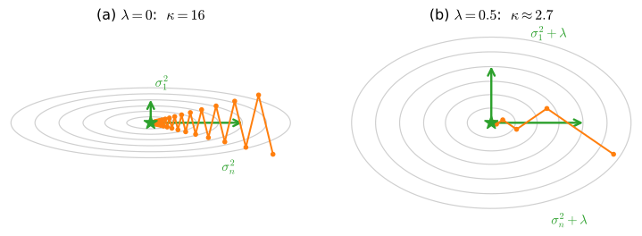
Geometrically, a large \(\kappa\) produces highly elongated level sets of \(\|\mathbf{A}\mathbf{x}-\mathbf{b}\|^2\). This is the same narrow-valley geometry shown in Figure 24.3.5: it makes a linear solve sensitive and slows gradient descent.
26.5.4.3 Conditioning of the Normal Equations
Least squares illustrates how an algebraically equivalent formulation can worsen conditioning. The normal equations for \(\min_{\mathbf{w}}\|\mathbf{A}\mathbf{w}-\mathbf{b}\|^2\) are \(\mathbf{A}^\top\mathbf{A}\mathbf{w}=\mathbf{A}^\top\mathbf{b}\). Solving this system depends on \(\kappa(\mathbf{A}^\top\mathbf{A})\) rather than \(\kappa(\mathbf{A})\). As shown in Section 24.3.3.2, for any full-column-rank matrix \(\mathbf{A}\),
\[ \kappa(\mathbf{A}^\top\mathbf{A}) = \kappa(\mathbf{A})^2 , \tag{26.5.10}\]
because \(\mathbf{A}^\top\mathbf{A}=\mathbf{V}\boldsymbol{\Sigma}^2\mathbf{V}^\top\) has singular values \(\sigma_i^2\) (Section 24.3.1.2). The normal equations can therefore lose about \(2\log_{10}\kappa\) decimal digits, whereas an SVD- or QR-based method that operates directly on \(\mathbf{A}\) loses about \(\log_{10}\kappa\). QR writes \(\mathbf{A}=\mathbf{Q}\mathbf{R}\) with \(\mathbf{Q}\) orthonormal and \(\mathbf{R}\) triangular, as illustrated in Section 24.1. For \(\kappa(\mathbf{A})=10^5\), the predicted difference is about five digits:
rng = np.random.default_rng(1)
m, n = 100, 10
U, _ = np.linalg.qr(rng.normal(size=(m, n)))    # random orthonormal columns
V, _ = np.linalg.qr(rng.normal(size=(n, n)))
sigma = np.logspace(0, -5, n)                   # kappa(A) = 10^5 by design
A = U * sigma @ V.T                             # A = U diag(sigma) V^T
w_true = rng.normal(size=n)
b = A @ w_true
print(f'kappa(A) = {np.linalg.cond(A):.1e}   '
      f'kappa(A^T A) = {np.linalg.cond(A.T @ A):.1e}')
w_ne = np.linalg.solve(A.T @ A, A.T @ b)        # normal equations
w_svd = np.linalg.lstsq(A, b, rcond=None)[0]    # SVD-based solve
for name, w in [('normal equations', w_ne), ('SVD (lstsq)     ', w_svd)]:
    err = np.linalg.norm(w - w_true) / np.linalg.norm(w_true)
    print(f'{name}: relative error {err:.1e}  '
          f'({-np.log10(err):.1f} correct digits)')
kappa(A) = 1.0e+05 kappa(A^T A) = 1.0e+10
normal equations: relative error 7.7e-08 (7.1 correct digits)
SVD (lstsq) : relative error 5.5e-14 (13.3 correct digits)The experiment gives \(\kappa(\mathbf{A}^\top\mathbf{A})=10^{10}\), the square of \(\kappa(\mathbf{A})=10^5\). The normal equations recover about seven correct digits, compared with roughly 13 for the SVD-based solve. The difference of five to six digits agrees with the predicted \(\log_{10}\kappa=5\). Numerical libraries therefore implement least-squares solves with QR or SVD, as in lstsq. For the same reason, Section 24.3.3.1 constructs the pseudoinverse from the SVD rather than from \((\mathbf{A}^\top\mathbf{A})^{-1}\mathbf{A}^\top\).
26.5.4.4 Ridge Regularization as Preconditioning
When \(\kappa(\mathbf{A})\) itself is the problem (nearly collinear features, a rank-deficient design), no choice of route saves the original problem. A preconditioner transforms a problem to reduce its condition number without changing its solution; the per-coordinate rescalings of Section 26.2 apply the same idea inside an optimizer. Ridge regularization conditions the problem the way a preconditioner does, with one difference we return to below: it changes the problem, and it changes it in exactly the right direction. Minimizing \(\|\mathbf{A}\mathbf{w} - \mathbf{b}\|^2 + \lambda \|\mathbf{w}\|^2\) yields
\[ \mathbf{w}_\lambda = (\mathbf{A}^\top\mathbf{A} + \lambda \mathbf{I})^{-1} \mathbf{A}^\top \mathbf{b}, \tag{26.5.11}\]
and the added \(\lambda\mathbf{I}\) acts directly on the spectrum.
Proposition (ridge improves conditioning monotonically). Let \(\mathbf{A}\) have singular values \(\sigma_1 \ge \cdots \ge \sigma_n \ge 0\). For every \(\lambda > 0\) the matrix \(\mathbf{A}^\top\mathbf{A} + \lambda\mathbf{I}\) is symmetric positive definite (hence invertible, even when \(\mathbf{A}\) is rank deficient), with
\[ \kappa(\mathbf{A}^\top\mathbf{A} + \lambda\mathbf{I}) = \frac{\sigma_1^2 + \lambda}{\sigma_n^2 + \lambda}, \tag{26.5.12}\]
which is strictly decreasing in \(\lambda\) whenever \(\sigma_1 > \sigma_n\) and tends to \(1\) as \(\lambda \to \infty\).
Proof. Writing \(\mathbf{A}^\top\mathbf{A} = \mathbf{V}\boldsymbol{\Sigma}^2\mathbf{V}^\top\) as above, \(\mathbf{A}^\top\mathbf{A} + \lambda\mathbf{I} = \mathbf{V}(\boldsymbol{\Sigma}^2 + \lambda\mathbf{I})\mathbf{V}^\top\): the same eigenvectors, every eigenvalue shifted up to \(\sigma_i^2 + \lambda \ge \lambda > 0\). Positive definiteness and Equation 26.5.12 follow. For monotonicity, with \(a = \sigma_1^2 > b = \sigma_n^2\),
\[ \frac{d}{d\lambda} \frac{a + \lambda}{b + \lambda} = \frac{b - a}{(b + \lambda)^2} < 0, \]
and as \(\lambda \to \infty\) the ratio tends to \(1\). \(\blacksquare\)
Adding \(\lambda\mathbf{I}\) lifts the floor of the spectrum while barely moving its ceiling. The resulting level sets are less elongated, as Figure 26.5.2 shows. The solve in Equation 26.5.11 becomes more accurate (fewer digits lost, by the rule of thumb), and gradient descent on the ridge objective becomes faster, since its contraction factor is the \((\kappa - 1)/(\kappa + 1)\) we derived in Section 26.1. The cell below measures both at once: for each \(\lambda\) it computes Equation 26.5.12 and runs gradient descent to a fixed relative tolerance of \(10^{-6}\), counting iterations.
rng = np.random.default_rng(2)
m, n = 200, 20
U, _ = np.linalg.qr(rng.normal(size=(m, n)))
V, _ = np.linalg.qr(rng.normal(size=(n, n)))
sigma = np.logspace(0, -2, n)                   # kappa(A) = 100
A = U * sigma @ V.T
b = A @ rng.normal(size=n)

def gd_iterations(lam, tol=1e-6):
    """Iterations for GD on the ridge objective to reach tol."""
    M, g = A.T @ A + lam * np.eye(n), A.T @ b
    w_star = np.linalg.solve(M, g)
    mu, L = sigma.min()**2 + lam, sigma.max()**2 + lam
    eta, w = 2.0 / (L + mu), np.zeros(n)        # optimal fixed step size
    for k in range(1, 200_000):
        w -= eta * (M @ w - g)
        if np.linalg.norm(w - w_star) <= tol * np.linalg.norm(w_star):
            return k

lams = np.logspace(-4, 0, 9)
kappas = (sigma.max()**2 + lams) / (sigma.min()**2 + lams)
iters = np.array([gd_iterations(lam) for lam in lams])
print('iterations / kappa:', (iters / kappas).round(2))
d2l.plot(lams, [kappas, iters.astype(float)], 'lambda', None,
         legend=['kappa(A^T A + lambda I)', 'GD iterations to 1e-6'],
xscale='log', yscale='log')iterations / kappa: [5.89 5.9 5.94 5.99 6.06 6.15 6.19 6.25 6. ]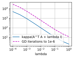
iterations / kappa: [5.89 5.9 5.94 5.99 6.06 6.15 6.19 6.25 6. ]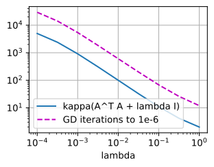
iterations / kappa: [5.89 5.9 5.94 5.99 6.06 6.15 6.19 6.25 6. ]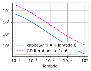
iterations / kappa: [5.89 5.9 5.94 5.99 6.06 6.15 6.19 6.25 6. ]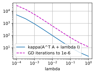
The two curves fall together across four orders of magnitude of \(\lambda\), from \(\kappa \approx 5000\) and roughly \(29{,}000\) iterations at \(\lambda = 10^{-4}\) down to \(\kappa = 2\) and a dozen iterations at \(\lambda = 1\), and the printed ratio sits between \(5.89\) and \(6.25\) throughout: iteration count is a constant multiple of \(\kappa\), the constant being about \(\tfrac12 \ln(1/\textrm{tol}) \approx 6.9\) predicted by the \((\kappa - 1)/(\kappa + 1)\) contraction (slightly less here because a random initial error is not perfectly aligned with the slowest eigendirection). Ridge thus conditions the problem exactly as a preconditioner would, with one difference: a true preconditioner leaves the minimizer unchanged, while ridge biases the solution, shrinking \(\mathbf{w}_\lambda\) toward \(\mathbf{0}\); Section 26.4 showed the precise sense in which the penalty \(\lambda\|\mathbf{w}\|^2\) is the Lagrangian counterpart of a norm constraint. Thus a regularization parameter chosen for statistical reasons can also improve the conditioning of the linear algebra and the convergence rate of gradient descent.
26.5.5 Summary
- A floating-point format has finite relative precision, absolute spacing that doubles at each power of two, and finite overflow and underflow thresholds. Loss scaling protects fp16 gradients from underflow; bfloat16 exchanges mantissa precision for fp32’s exponent range; fp8 formats generally require explicit tensor- or block-level scaling.
- Softmax is shift invariant, so subtracting the largest logit before exponentiation prevents overflow for finite logits. Cross-entropy should be computed directly from logits as \(\mathrm{lse}(\mathbf{z})-z_y\); forming probabilities first can produce
inf,NaN, or a silently clipped gradient. - Subtracting nearby values can amplify existing relative error by \((|a|+|b|)/|a-b|\). Stable alternatives include
log1pandexpm1near zero and Welford’s recursion for one-pass variance. - Backward error measures how much the input must change to make a computed result exact. The condition number converts this perturbation into forward error, so a backward-stable solve can lose about \(\log_{10}\kappa\) decimal digits on an ill-conditioned problem.
- The normal equations square the condition number: \(\kappa(\mathbf{A}^\top\mathbf{A})=\kappa(\mathbf{A})^2\). Ridge regularization changes it to \((\sigma_1^2+\lambda)/(\sigma_n^2+\lambda)\), improving both numerical conditioning and the fixed-step gradient-descent rate.
26.5.6 Exercises
- Compute \(\varepsilon_{\text{mach}}\) for float32 by a halving loop: start from \(e = 1\) and halve until \(1 + e == 1\) in float32. Why does the loop exit at \(e = 2^{-24}\) rather than at \(2^{-23}\), and how does that relate to the unit roundoff \(u\) in Equation 26.5.2? Repeat the loop with bfloat16 arithmetic (emulated or native) and confirm \(2^{-7}\).
- Find all integer logits \(x\) for which \(e^x\) overflows in fp16 but not in fp32. A network’s final layer emits activations of size \(\approx 30\): explain, with the numbers from this section, why training it in fp16 without loss scaling fails even though the softmax probabilities are perfectly representable.
- Prove that \(\nabla\, \mathrm{lse}(\mathbf{z}) = \mathrm{softmax}(\mathbf{z})\) and use Section 26.3 to conclude that lse is convex. Then show that the cross-entropy Equation 26.5.6 has gradient \(\mathrm{softmax}(\mathbf{z}) - \mathbf{e}_y\), another reason to compute the loss from logits.
- Construct a small dataset (three numbers suffice) for which the naive variance formula returns a strictly negative number in float64, and verify that Welford’s recursion Equation 26.5.8 gets it right. Then derive the pairwise merge rule: given \((m, M, k)\) for two disjoint batches, express the combined statistics exactly; this is how the computation parallelizes across devices.
- Show that if \(a\) and \(b\) carry relative errors of size \(u\), the relative error of the computed \(a - b\) can be as large as \((|a| + |b|)\,u / |a - b|\), and that the subtraction itself adds no rounding error when \(a/2 \le b \le 2a\) (Sterbenz’s lemma (Sterbenz 1974); prove it for floats with the same exponent).
- Rewrite each of the following to avoid cancellation, and check one of them numerically in float32: \(\sqrt{x + 1} - \sqrt{x}\) for large \(x\); \(1 - \cos x\) for small \(x\); the smaller root of \(ax^2 + bx + c = 0\) when \(b^2 \gg 4ac\).
- For the Hilbert experiment, compute the backward error of each solve with respect to the right-hand side, \(\|\mathbf{H}\hat{\mathbf{x}} - \mathbf{b}\|/\|\mathbf{b}\|\), and verify that the forward error is bounded by Equation 24.3.13 applied to that perturbation. Where in the table is the bound tightest?
- Let \(\mathbf{A}\) have \(\sigma_1 = 1\) and \(\sigma_n = 10^{-3}\). Using Equation 26.5.12 and the GD contraction factor \((\kappa - 1)/(\kappa + 1)\) from Section 26.1, compute the condition number and the predicted iteration count (to relative error \(10^{-6}\)) for \(\lambda \in \{0, 10^{-4}, 10^{-2}\}\). Then explain, via Section 26.4, which constrained problem each \(\lambda\) implicitly solves.
26.5.7 Discussions
The condition number governs both the convergence rate of fixed-step gradient descent (Section 26.1) and the sensitivity of a linear solve. Ridge regularization, which corresponds to a norm constraint through the Lagrangian analysis in Section 26.4, can improve both.
The same stable computations recur elsewhere in the book. Softmax and attention use maximum subtraction and log-sum-exp; naive Bayes and other probabilistic calculations use log-space arithmetic (Section 27.7); and batch normalization uses stable running moments. Section 4.4 studies vanishing and exploding gradients through products of Jacobians, while Chapter 29 examines the propagation of error and noise in continuous-time models. Higham (2002) provides a comprehensive treatment of numerical error analysis for the underlying linear-algebra algorithms.