import math
import re
import zlib
import numpy as np
from d2l import torch as d2l28.2 Codes, Compression, and Perplexity
Section 28.1 read every log-loss as a code length: a model whose loss on a text is \(x\) bits per symbol should be able to store that text in about \(x\) bits per symbol. We never built the code that does this, and the reading means little until such a code exists. This section asks two questions: is there a code whose length is a model’s log-loss, and how close do real compressors come to it?
Compressors are familiar tools, and they already suggest the answer. Take The Time Machine, the novel of Section 8.2, reduced to 173,428 characters over 27 symbols, the 26 letters and the space. The general-purpose compressor zlib stores it in \(2.84\) bits per character. A small model that predicts each character from the three before it, learning its counts as it reads, codes the same text in \(2.55\) bits per character. The model that predicts the text better also writes the shorter file, and this section shows why. Once a code exists whose length is the log-loss, a loss of \(1.8\) nats per token is a file size, a perplexity is a branching factor, and choosing between two models becomes a question of which complete description is shorter.
We build the code in steps. A code that needs no separators between its codewords has a fixed budget of short codewords to hand out. The best length for a symbol of probability \(p\) is \(\log_2(1/p)\) bits, and rounding these lengths to whole bits costs up to one bit per symbol. Coding the whole message as one unit rounds only once. For a source with memory, such as text, the long-run floor is the entropy rate, and perplexity is the per-token loss exponentiated.
The section rests on one fact from the previous section. The expected log-loss of a model \(Q\) on data from \(P\), the cross-entropy, splits into the entropy of the data and the Kullback–Leibler divergence,
\[ \textrm{CE}_2(P, Q) = -\sum_i p_i \log_2 q_i = H_2(P) + D_{\textrm{KL}}^{(2)}(P \| Q), \qquad D_{\textrm{KL}}^{(2)}(P \| Q) \geq 0, \]
with equality in the last inequality only when \(Q = P\) (Gibbs’ inequality). Thus a model can never beat the entropy of the data, and it reaches the entropy only by matching the data distribution. For the running pair \(P = (0.6, 0.3, 0.1)\) and \(Q = (0.2, 0.5, 0.3)\) the three terms are \(1.867 = 1.295 + 0.571\) bits.
This section works in bits because codewords are binary strings. The subscript \(2\) and the superscript \((2)\) mark base-\(2\) logarithms, and a quantity of \(x\) bits is \(x \ln 2\) nats (\(1\) bit \(= 0.693\) nats). For a coin with bias \(p\) we write \(H_2(p, 1-p) = H_b(p)/\ln 2\), its binary entropy in bits.
We use the following imports throughout the section.
import math
import re
import zlib
import numpy as np
from d2l import tensorflow as d2l
import math
import re
import zlib
import numpy as np
from d2l import jax as d2limport math
import re
import zlib
import numpy as np
from d2l import mxnet as d2l28.2.1 Symbol Codes
We must send a stream of symbols, drawn independently from a distribution \(P\) over \(k\) outcomes, as one binary string with no separators, and the receiver must split it back into symbols.
28.2.1.1 Prefix Codes and the Kraft Inequality
Each outcome \(i\) gets a binary string, its codeword, of length \(\ell_i\). The receiver can split the stream without separators if no codeword is a prefix of another; such a code is called prefix-free, or a prefix code. Telephone numbers work this way: once the dialed digits match a number, no longer number starts with the same digits, so the exchange knows that the number is complete. The code \(0, 10, 110, 111\) for four symbols is prefix-free, and the stream 110010111 splits in only one way, as 110|0|10|111.

Figure 28.2.1 draws this code as a binary tree. A codeword of length \(\ell\) ends at a leaf and removes everything below it, a fraction \(2^{-\ell}\) of the tree. The fractions removed by all codewords must fit into one tree, a budget of \(1\), so short codewords are expensive. The lengths \((1, 2, 3, 3)\) of the figure use \(\tfrac12 + \tfrac14 + \tfrac18 + \tfrac18 = 1\), the whole tree. Four codewords of length \(1\) would use \(2\) trees, which is impossible: only two strings of length one exist. The lengths \((1, 2, 4)\) use \(\tfrac12 + \tfrac14 + \tfrac1{16} = 0.8125\) and fit with room to spare, for instance as \(0, 10, 1100\).
Proposition (Kraft inequality). A prefix-free binary code with codeword lengths \(\ell_1, \ldots, \ell_k\) exists if and only if
\[ \sum_{i=1}^k 2^{-\ell_i} \leq 1. \tag{28.2.1}\]
Proof. Identify each codeword \(c\) of length \(\ell\) with the half-open interval \([0.c,\, 0.c + 2^{-\ell})\) of all real numbers in \([0, 1)\) whose binary expansion begins with \(c\). For example, the codeword \(10\) owns \([0.10_2, 0.11_2) = [\tfrac{1}{2}, \tfrac{3}{4})\), of length \(2^{-2}\). Such dyadic intervals are either nested or disjoint. If \(c\) is a prefix of \(c'\), every number that begins with \(c'\) begins with \(c\), so the intervals are nested. Otherwise \(c\) and \(c'\) differ at some digit within the shorter length, no number can begin with both, and the intervals are disjoint. A prefix-free code therefore owns disjoint intervals inside \([0, 1)\), and their total length \(\sum_i 2^{-\ell_i}\) is at most \(1\).
Conversely, let the lengths satisfy Equation 28.2.1. The key step is to sort them, \(\ell_1 \leq \cdots \leq \ell_k\), and to lay intervals of length \(2^{-\ell_i}\) side by side from \(0\). The \(i\)-th interval starts at \(s_i = \sum_{m < i} 2^{-\ell_m}\) and ends at \(s_i + 2^{-\ell_i} \leq 1\). Every earlier length satisfies \(\ell_m \leq \ell_i\), so each term of \(s_i\) is a multiple of \(2^{-\ell_i}\), and so is \(s_i\). The \(i\)-th interval is therefore the dyadic interval of the codeword formed by the first \(\ell_i\) binary digits of \(s_i\). The intervals are disjoint, so by the first part no codeword is a prefix of another. \(\blacksquare\)
Thus codeword lengths are a budget: each codeword of length \(\ell\) spends \(2^{-\ell}\), and a prefix code can spend at most \(1\). A code is uniquely decodable if every concatenation of codewords parses in only one way, prefix-free or not. McMillan showed that such codes obey the same inequality (McMillan 1956) (Exercise 3). Every length profile that a uniquely decodable code achieves, a prefix code therefore achieves too, and restricting to prefix codes costs nothing.
28.2.1.2 Shannon Lengths and the Entropy Bound
Given the budget, which lengths minimize the expected code length \(\mathbb{E}[\ell] = \sum_i p_i \ell_i\)? Frequent symbols should get short codewords, but a codeword of length \(1\) already spends half the budget.
To see where the answer comes from, let the lengths be real numbers for a moment. Unspent budget never helps, because shortening a codeword lowers \(\mathbb{E}[\ell]\), so at the optimum \(\sum_i 2^{-\ell_i} = 1\). Lagrange’s rule for a minimum under an equality constraint says that there the gradient of the objective is a multiple of the gradient of the constraint (Section 25.2.2.5). The derivative of \(\mathbb{E}[\ell]\) in \(\ell_i\) is \(p_i\), and that of \(\sum_i 2^{-\ell_i}\) is \(-2^{-\ell_i}\ln 2\). Hence \(p_i = \lambda\, 2^{-\ell_i} \ln 2\) for one constant \(\lambda\) and all \(i\), so \(2^{-\ell_i}\) is proportional to \(p_i\). The constraint fixes the constant to \(1\), and the best real lengths and their expected length are
\[ \ell_i = \log_2 \frac{1}{p_i}, \qquad \mathbb{E}[\ell] = \sum_i p_i \log_2 \frac{1}{p_i} = H_2(P). \]
So each symbol gets as many bits as its surprisal, and the expected length is the entropy. Real codewords need whole bits. For the dyadic source \(P = (\tfrac12, \tfrac14, \tfrac18, \tfrac18)\) the surprisals \(1, 2, 3, 3\) are already integers, the code of Figure 28.2.1 has these lengths, and \(\mathbb{E}[\ell] = 1.75\) bits \(= H_2(P)\), with nothing wasted. For the running \(P = (0.6, 0.3, 0.1)\) the surprisals are \(0.74\), \(1.74\) and \(3.32\) bits. Rounding them up gives the Shannon lengths \(1, 2, 4\), the profile that fit the tree with room to spare. Its Kraft sum is \(0.8125\), and \(\mathbb{E}[\ell] = 0.6 + 0.6 + 0.4 = 1.6\) bits, against \(H_2(P) = 1.295\).
Proposition (entropy bounds the code length). Let \(P\) have all \(p_i > 0\) (symbols of probability zero need no codeword). Every prefix-free binary code has \(\mathbb{E}[\ell] \geq H_2(P)\), with equality if and only if every \(p_i\) equals \(2^{-\ell_i}\). The Shannon code with lengths \(\ell_i = \lceil \log_2 (1/p_i) \rceil\) is prefix-free and has \(\mathbb{E}[\ell] < H_2(P) + 1\).
Proof. For the lower bound, compare the code with the distribution it implies. Let \(Z = \sum_i 2^{-\ell_i}\), which is at most \(1\) by Kraft, and let \(q_i = 2^{-\ell_i}/Z\). Then \(\ell_i = -\log_2 q_i - \log_2 Z\), and averaging under \(P\) gives
\[ \mathbb{E}[\ell] = \sum_i p_i \ell_i = -\sum_i p_i \log_2 q_i - \log_2 Z = H_2(P) + D_{\textrm{KL}}^{(2)}(P \| Q) - \log_2 Z \geq H_2(P). \tag{28.2.2}\]
The inequality holds because the KL term is never negative and \(-\log_2 Z \geq 0\). Equality needs both to vanish: \(Q = P\) and \(Z = 1\), that is, \(p_i = 2^{-\ell_i}\). For the upper bound, the Shannon lengths satisfy \(2^{-\ell_i} \leq p_i\), so they pass Kraft’s test (\(\sum_i 2^{-\ell_i} \leq \sum_i p_i = 1\)) and a prefix code with these lengths exists. Each length is less than \(\log_2(1/p_i) + 1\), and averaging gives \(\mathbb{E}[\ell] < H_2(P) + 1\). \(\blacksquare\)
Thus every code wastes bits in two ways: by implying a distribution \(Q\) other than \(P\), and by leaving budget unspent. On the running pair the Shannon code wastes \(1.6 - 1.295 = 0.305\) bits, of which \(0.005\) is mismatch and \(0.300\) is unspent budget (Exercise 4). The entropy therefore determines the best expected length to within one bit per symbol, and the two are equal only for dyadic probabilities.
The one bit is not an artifact of the proof. The best symbol code, built by Huffman’s algorithm (Huffman 1952), gives the pair the lengths \(1, 2, 2\) and \(1.4\) bits (Exercise 2). No symbol code can go below one bit per symbol, however, because no codeword is shorter than one bit. This matters most for a skewed source. Take one that emits the symbol a with probability \(0.9\) and the symbol b with probability \(0.1\). Its entropy is \(0.47\) bits per symbol, and each a carries only \(\log_2(1/0.9) = 0.15\) bits of surprise. Yet every symbol code spends at least one whole bit on an a, more than six times its information, and so at least \(1\) bit per symbol against an entropy of \(0.47\). The “\(+1\)” is the cost of coding one symbol at a time. Coding blocks of symbols shrinks it: Huffman’s code for pairs of a/b symbols spends \(0.645\) bits per symbol, and long blocks drive the slack to zero (Cover and Thomas 1999).
28.2.1.3 Mismatched Codes and Cross-Entropy
In practice the code is built from a model \(Q\), and the data come from \(P\). The Shannon code for \(Q\) has lengths \(\ell_i = \lceil \log_2 (1/q_i) \rceil\), which requires \(q_i > 0\) for every symbol that \(P\) can produce. On data from \(P\) its expected length satisfies
\[ \textrm{CE}_2(P, Q) \;\leq\; \mathbb{E}_P[\ell] \;<\; \textrm{CE}_2(P, Q) + 1, \qquad \textrm{CE}_2(P, Q) = -\sum_i p_i \log_2 q_i = H_2(P) + D_{\textrm{KL}}^{(2)}(P \| Q). \tag{28.2.3}\]
Proof. Termwise, \(\log_2(1/q_i) \leq \ell_i < \log_2(1/q_i) + 1\). Average under \(P\). \(\blacksquare\)
Thus cross-entropy is the length of a code built from the model, and KL is the extra length over the code built from the truth. For the running pair, the Shannon lengths for \(Q = (0.2, 0.5, 0.3)\) are \(3, 1, 2\), and on data from \(P\) they average \(1.8 + 0.3 + 0.2 = 2.3\) bits, inside the window \(1.867 \leq 2.3 < 2.867\). The dyadic source coded with the uniform codebook, two bits for every symbol, costs \(2.0 = 1.75 + 0.25\) bits. This is the matched length plus \(D_{\textrm{KL}}^{(2)}(P \| U) = 0.25\), where \(U\) is the uniform distribution on the four symbols.
How long are the Shannon codes for the two running sources, and what does the wrong code cost? The cell builds each code from the distribution it is given and averages its lengths under the data distribution.
def shannon_lengths(q):
    return [math.ceil(math.log2(1 / q_i)) for q_i in q]

def code_report(name, p, q):
    """The Shannon code built from q, used on data from p (all in bits)."""
    ells = shannon_lengths(q)
    kraft = sum(2 ** -ell for ell in ells)
    avg = sum(p_i * ell for p_i, ell in zip(p, ells))
    ce2 = -sum(p_i * math.log2(q_i) for p_i, q_i in zip(p, q))
    print(f'{name:<16} lengths {ells}  Kraft {kraft:.4f}  '
          f'E[ell] {avg:.3f}  CE2 {ce2:.3f}')

dyadic, uniform = [1/2, 1/4, 1/8, 1/8], [1/4] * 4
p, q = [0.6, 0.3, 0.1], [0.2, 0.5, 0.3]
code_report('dyadic, own', dyadic, dyadic)
code_report('dyadic, uniform', dyadic, uniform)
code_report('P, own', p, p)
code_report('P, code from Q', p, q)
dyadic, own lengths [1, 2, 3, 3] Kraft 1.0000 E[ell] 1.750 CE2 1.750
dyadic, uniform lengths [2, 2, 2, 2] Kraft 1.0000 E[ell] 2.000 CE2 2.000
P, own lengths [1, 2, 4] Kraft 0.8125 E[ell] 1.600 CE2 1.295
P, code from Q lengths [3, 1, 2] Kraft 0.8750 E[ell] 2.300 CE2 1.867When the code is built from the data distribution, the column CE2 is the entropy. The dyadic source wastes nothing, and the uniform codebook costs it \(0.25\) bits. The pair’s own Shannon code spends \(1.6\) bits against an entropy of \(1.295\), and the code from \(Q\) spends \(2.3\), inside its one-bit window above the cross-entropy \(1.867\).
The bound Equation 28.2.3 covers the Shannon code of \(Q\), not every code someone might build from \(Q\). Huffman’s code for \(Q\) has lengths \(2, 1, 2\) and costs \(1.2 + 0.3 + 0.2 = 1.7 < 1.867\) bits on data from \(P\). Its implied distribution is \((\tfrac14, \tfrac12, \tfrac14)\), not \(Q\), and it happens to be closer to \(P\). Every code implies a distribution, \(2^{-\ell_i}/Z\), and its expected length on \(P\) is the cross-entropy of \(P\) with that distribution, plus any unspent budget \(-\log_2 Z\).
28.2.2 Stream Codes
28.2.2.1 Arithmetic Coding
The ceiling in \(\ell_i = \lceil \log_2(1/p_i) \rceil\) rounds a fraction of a bit up to a whole bit once per symbol. For a skewed source the rounding dominates the code length: the a of probability \(0.9\) carries \(0.15\) bits and costs \(1\). The remedy is to stop coding symbols and to code the whole message as one interval. A code that assigns one codeword to a whole message, rather than one to each symbol, is a stream code. Arithmetic coding (Rissanen 1976; Witten et al. 1987) is the standard stream code, and Figure 28.2.2 shows it on the message aaaaaaaaba.
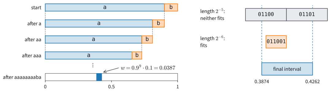
The coder keeps a current interval, initially \([0, 1)\). To encode the next symbol it splits the current interval into one slice per possible symbol, with widths proportional to the model’s conditional probabilities \(q(\cdot \mid x_{<i})\), and keeps the slice of the symbol that occurred. Each step multiplies the width by the probability of the observed symbol, so after the message \(x_1, \ldots, x_n\) the interval has width
\[ w = \prod_{i=1}^n q(x_i \mid x_{<i}), \]
the probability that the model assigns to the whole message. The final interval identifies the message: a decoder that replays the model sees which slice the transmitted number falls into, recovers each symbol in turn, and narrows its own interval in step. The decoder must also know \(n\), or the model must include an end-of-message symbol, and we do not count either cost here. What remains is to name a point of the final interval in binary, and the dyadic intervals of the Kraft proof do this.
Any interval of width \(w\) contains a dyadic interval of length \(2^{-\ell}\) when \(\ell = \lceil \log_2(1/w) \rceil + 1\). Then \(2^{-\ell} \leq w/2\), so the first multiple of \(2^{-\ell}\) at or above the interval’s left end lies in its left half, and the cell of length \(2^{-\ell}\) starting there ends inside the interval. Panel (b) of Figure 28.2.2 shows both sides of this: the cells of length \(2^{-5}\) stick out of the final interval, while one cell of length \(2^{-6}\) fits. Since \(\ell < \log_2(1/w) + 2\), the codeword length satisfies
\[ \ell \;<\; \sum_{i=1}^n \log_2 \frac{1}{q(x_i \mid x_{<i})} + 2, \tag{28.2.4}\]
the message’s total surprisal under the model plus at most two bits, for a message length \(n\) known to the decoder. Thus the rounding happens once per message, not once per symbol. The codewords of different messages of length \(n\) lie in disjoint message intervals, so they form a prefix code, and the entropy bound applies to them as a code for whole messages.
What do the coder’s interval and codeword look like for aaaaaaaaba, and what does the symbol-by-symbol Shannon code spend on the same message? The cell narrows the interval, constructs the codeword from the interval’s ends, and checks that its dyadic cell lies inside.
msg = 'aaaaaaaaba'                    # nine a's, one b
q = {'a': 0.9, 'b': 0.1}              # an i.i.d. model of the source

lo, hi = 0.0, 1.0
for ch in msg:                        # keep the observed symbol's slice
    width = hi - lo
    if ch == 'a':                     # 'a' owns the left 90% of the interval
        hi = lo + width * q['a']
    else:                             # 'b' owns the right 10%
        lo = lo + width * q['a']

ell = math.ceil(-math.log2(hi - lo)) + 1      # codeword length
m = math.ceil(lo * 2 ** ell)                  # first multiple of 2^-ell >= lo
assert lo <= m / 2 ** ell and (m + 1) / 2 ** ell <= hi
surprisal = -math.log2(math.prod(q[ch] for ch in msg))
shannon_bits = sum(math.ceil(math.log2(1 / q[ch])) for ch in msg)
print(f'final interval [{lo:.4f}, {hi:.4f}), width {hi - lo:.4f}')
print(f'surprisal {surprisal:.2f} bits, codeword {m:0{ell}b} ({ell} bits)')
print(f'symbol-by-symbol Shannon code: {shannon_bits} bits')
final interval [0.3874, 0.4262), width 0.0387
surprisal 4.69 bits, codeword 011001 (6 bits)
symbol-by-symbol Shannon code: 13 bitsThe final width \(0.0387\) is the product \(0.9^9 \cdot 0.1\), as the construction promises. The message has \(4.69\) bits of surprisal and the arithmetic code spends \(6\) bits on it, the codeword 011001, while the symbol-by-symbol code spends \(13\), a whole bit on each of the nine cheap a’s. This message has the source’s typical composition, nine a’s and one b, so its surprisal equals \(10\, H_2(0.9, 0.1) = 4.69\) bits. A message with two b’s would cost more. On long messages the two extra bits vanish into the total, and the code length per symbol approaches the model’s log-loss per symbol.
Floating-point narrowing works only for short messages. The width shrinks by a factor \(q\) at every step, and after about a hundred symbols the ends of the interval can no longer be told apart in the \(53\)-bit significand of a double (Exercise 5). Practical coders use integer arithmetic and emit the leading bits as soon as both ends agree on them, which keeps the working interval at a fixed precision (Witten et al. 1987). Either way, the code length of a message is its log-loss to within two bits, so \(n\) times a model’s per-symbol cross-entropy in bits is a file size.
28.2.2.2 A Language Model as a Compressor
Nothing in the construction required independent symbols. Any conditional model \(q(\cdot \mid x_{<i})\) drives the coder, provided the encoder and the decoder compute the same probabilities, bit for bit in finite precision. An autoregressive language model with an arithmetic coder is therefore a lossless compressor. With a shared tokenizer, model and coder, the code length of a document is its total surprisal under the model plus at most two bits. A file format adds framing, and the model itself must be shared once, which this length does not count.
The smallest model that learns is a counting model. An adaptive order-\(m\) model predicts each character from the \(m\) characters before it, its context \(s\), with
\[ q(x \mid s) = \frac{c(s, x) + \tfrac12}{c(s) + \tfrac{k}{2}}, \]
where \(c(s, x)\) counts how often \(x\) has followed \(s\) so far, \(c(s) = \sum_x c(s, x)\), and \(k\) is the alphabet size. The half counts keep every probability positive, so no character ever costs infinitely many bits. After coding a character, the model adds it to the counts. The decoder repeats the same counting on the characters it has decoded, so the encoder never sends any parameters.
How many bits per character does such a model need for The Time Machine, the text of Section 8.2, and how does it compare with zlib? The first cell loads the text, keeps letters and spaces, and defines the adaptive code length in bits per character.
fname = d2l.download(d2l.DATA_URL + 'timemachine.txt',
                     sha1_hash='090b5e7e70c295757f55df93cb0a180b9691891a')
with open(fname) as f:
    text = re.sub('[^A-Za-z]+', ' ', f.read()).lower()   # 26 letters, space

def adaptive_bits(text, m, k):
    """Bits per character of the adaptive order-m model with half counts."""
    counts, totals, bits = {}, {}, 0.0
    for i, ch in enumerate(text):
        s = text[max(0, i - m):i]                # the context
        c = counts.setdefault(s, {})
        bits -= math.log2((c.get(ch, 0) + 0.5) / (totals.get(s, 0) + k / 2))
        c[ch] = c.get(ch, 0) + 1                 # learn after coding
        totals[s] = totals.get(s, 0) + 1
    return bits / len(text)
The second cell codes the text with contexts of zero to four characters and compresses it with zlib at its highest level.
k = len(set(text))
print(f'{len(text)} characters over {k} symbols')
for m in range(5):
    print(f'order {m}: {adaptive_bits(text, m, k):.2f} bits/char')
print(f'zlib -9: {8 * len(zlib.compress(text.encode(), 9)) / len(text):.2f} '
      f'bits/char')
173428 characters over 27 symbols
order 0: 4.08 bits/char
order 1: 3.29 bits/char
order 2: 2.75 bits/char
order 3: 2.55 bits/char
order 4: 2.78 bits/char
zlib -9: 2.84 bits/charContext lowers the code length, from \(4.08\) bits per character with no context to \(2.55\) with three characters, which beats zlib’s \(2.84\). The four-character model loses to the three-character one, at \(2.78\) bits per character. Most of its \(27^4 \approx 530{,}000\) possible contexts are seen too rarely to learn their next-character distribution, and the bits spent while each context learns are part of the code length. The order-\(0\) length \(4.08\) agrees to two decimals with the entropy \(4.078\) of the text’s letter frequencies: learning \(26\) free frequencies costs about \(\tfrac{26}{2} \log_2 n \approx 226\) bits for the whole text, \(0.001\) bits per character. The cost of learning a model is the subject of the next subsection.
An adaptive model transmits no parameters, but it codes the early text poorly while it learns. A pretrained model codes every file well from the start, but its description must be shared once. Delétang et al. (2023) take the second route with a 70-billion-parameter language model. A coder driven by its next-token probabilities compresses ImageNet image patches to \(43.4\%\) of their raw size, against \(58.5\%\) for PNG, and LibriSpeech audio to \(16.4\%\), against \(30.3\%\) for FLAC.
28.2.2.3 Minimum Description Length
The richer of two models always fits the data at least as well: an order-\(4\) model fitted to the whole text has lower cross-entropy than an order-\(3\) model. Judged by the code length of the data alone, the richer model always wins. A receiver who does not have the model, however, must first be told it. The minimum description length (MDL) principle chooses the model \(\mathcal{M}\) with the shortest complete code, model and data together,
\[ \hat{\mathcal{M}} =\mathop{\mathrm{argmin}}_{\mathcal{M}} \bigl[L(\mathcal{M})+L(\mathcal{D}\mid \mathcal{M})\bigr], \tag{28.2.5}\]
where \(L(\mathcal{M})\) is the length of the model’s description in bits and \(L(\mathcal{D}\mid\mathcal{M})\) is the log-loss of the data \(\mathcal{D}\) under the model, a code length by the previous subsections. Thus a model must save more bits on the data than it costs to describe. MDL is Occam’s razor with simplicity measured in bits.
A coin makes the trade concrete. A sequence of \(n = 1{,}000\) flips shows \(600\) heads. The fair coin \(\mathcal{M}_0\) has nothing to describe, and it codes each flip in one bit: \(L(\mathcal{D} \mid \mathcal{M}_0) = 1{,}000\) bits. The model \(\mathcal{M}_1\), a coin with bias \(\theta\), must first send \(\theta\). Sending it to a precision of about \(1/\sqrt{n}\) costs \(L(\mathcal{M}_1) \approx \tfrac12 \log_2 1{,}000 \approx 5\) bits, and a finer precision would save fewer bits on the data than it costs to send (Exercise 7 derives the \(\tfrac12 \log_2 n\)).
The data then cost \(L(\mathcal{D} \mid \mathcal{M}_1) \approx 1{,}000\, H_2(0.6, 0.4) = 971\) bits. The total \(976 < 1{,}000\) selects the biased coin: it saves \(29\) bits on the data for \(5\) bits of parameter. With \(520\) heads the saving would be \(1.2\) bits, less than the \(5\), and MDL keeps the fair coin.
The compressor experiment above applied the same rule. The adaptive code length is a complete description, with the cost of learning the model inside it, and it selected the order-\(3\) model: the order-\(4\) model’s extra contexts cost more to learn than they saved.
MDL is close to Bayesian inference. Choosing \(L(\mathcal{M}) = -\log_2 P(\mathcal{M})\) and \(L(\mathcal{D}\mid\mathcal{M}) = -\log_2 P(\mathcal{D}\mid\mathcal{M})\) turns Equation 28.2.5 into the MAP objective. A one-part Bayesian code instead uses the marginal likelihood \(-\log_2\int P(\mathcal{D}\mid\theta)P(\theta)\,d\theta\), which averages over the parameter rather than sending one value.
A parameter count alone is not a description length. For a model with real-valued weights, a literal two-part code must also choose a precision for each weight, as the coin did. There, a parameter was worth its cost only if it saved more than about \(\tfrac12 \log_2 n\) bits on the data.
28.2.3 Entropy Rate and Typical Sequences
28.2.3.1 The Entropy Rate
How few bits per character can any code achieve on a source with memory, such as text? For independent symbols the floor is the entropy. Text is not independent: after q comes u. Let the source \(X_1, X_2, \ldots\) be stationary, meaning that the joint distribution of any block of symbols does not change when the block is shifted in time.
The best possible model of the next symbol is the source itself, and its expected log-loss is the conditional entropy of the next symbol given the past, \(H(X_n \mid X_{<n}) = \mathbb{E}\big[-\log_2 p(X_n \mid X_{<n})\big]\). The entropy rate is the limit of this loss, or equivalently of the entropy per symbol of long blocks,
\[ H_{\textrm{rate}} = \lim_{n \to \infty} \frac{1}{n} H(X_1, \ldots, X_n) = \lim_{n \to \infty} H(X_n \mid X_{<n}). \tag{28.2.6}\]
For a stationary source both limits exist and agree, and \(\tfrac1n H(X_1, \ldots, X_n)\) decreases monotonically to the limit (Cover and Thomas 1999). We grant these facts. Intuitively, each extra symbol of context can only help prediction, and the average of a nonincreasing sequence of losses is itself nonincreasing. For independent, identically distributed symbols both limits equal \(H(X_1)\).
The smallest source with memory is a two-state chain. Let it emit a or b, keep its current symbol with probability \(0.9\), and switch with probability \(0.1\). Both symbols are equally frequent, so a single symbol has entropy \(H(X_1) = 1\) bit. Given the previous symbol, the next is a coin of bias \(0.1\) from either state, so \(H(X_n \mid X_{n-1}) = H_2(0.9, 0.1)
= 0.47\) bits, and longer context adds nothing. Memory cuts the floor from \(1\) bit to \(0.47\). Exercise 8 does the general two-state chain.
For a stationary source no uniquely decodable code averages fewer than \(H_{\textrm{rate}}\) bits per symbol. A code for blocks of \(n\) symbols is a symbol code over the alphabet of blocks. The entropy bound, which extends to uniquely decodable codes by McMillan’s theorem, says that it spends at least \(H(X_1, \ldots, X_n)\) bits per block, and the monotone decrease gives \(H(X_1, \ldots, X_n) \geq n H_{\textrm{rate}}\). Dependence lowers this floor below the entropy of single symbols.
Shannon estimated the entropy rate of printed English at about one bit per character (Shannon 1951), far below the \(\log_2 27 = 4.75\) bits of uniformly random letters and spaces. The bits per character that a compressor achieves estimate an upper bound on the entropy rate, and the \(2.55\) of the order-\(3\) model is one such estimate. No compressor reports a lower bound.
28.2.3.2 Typical Sequences
The entropy bound concerns averages. What does one long message look like, and how many likely messages are there? Take independent bits that are \(1\) with probability \(0.3\), and messages of length \(n = 200\). All numbers are in bits.
The most probable message, all zeros, has probability \(0.7^{200} = 2^{-103}\). A message with \(60\) ones, the expected number, has probability \(0.3^{60}\, 0.7^{140} = 2^{-176.3}\), which is \(2^{-nH}\) with \(H = H_2(0.3, 0.7) = 0.881\) bits. There are \(\binom{200}{60} = 2^{172.2}\) such messages. The number of messages peaks at \(100\) ones, with \(2^{195.9}\) messages, but each of them has probability \(2^{-225}\), so together they carry only \(2^{-29}\) of the probability. Most messages are unlikely, and the most likely message is unrepresentative.
The surprisal per symbol of a message is a sample mean of independent surprisals, \(-\log_2 P(x_{1:n}) = \sum_i -\log_2 p(x_i)\), each with mean \(H = H_2(P)\). The law of large numbers says that such a mean converges in probability to its expectation:
\[ -\frac{1}{n}\log_2 P(X_{1:n}) =\frac{1}{n}\sum_{i=1}^n -\log_2 p(X_i) \xrightarrow{P} H. \tag{28.2.7}\]
Thus, for any fixed \(\delta > 0\), a long message has, with probability tending to one, surprisal within \(n\delta\) of \(nH\) bits. This is the asymptotic equipartition property (AEP). The messages it singles out form the typical set with tolerance \(\delta\) bits per symbol,
\[ A_\delta = \Big\{x_{1:n} :\ \Big|-\frac1n \log_2 P(x_{1:n}) - H\Big| < \delta\Big\}. \tag{28.2.8}\]
Proposition (AEP). Let \(X_1, \ldots, X_n\) be independent draws from a distribution \(P\) on a finite alphabet, with entropy \(H\) in bits, and let \(\delta > 0\). (i) \(P(A_\delta) \to 1\) as \(n \to \infty\). (ii) Every \(x_{1:n} \in A_\delta\) has \(2^{-n(H+\delta)} < P(x_{1:n}) < 2^{-n(H-\delta)}\). (iii) \(|A_\delta| \leq 2^{n(H+\delta)}\), and \(|A_\delta| \geq (1-\eta)\,2^{n(H-\delta)}\) whenever \(P(A_\delta) \geq 1-\eta\).
Proof. Part (i) is Equation 28.2.7, and part (ii) rewrites the definition of \(A_\delta\). For (iii), add the bounds of (ii) over the typical set: \(1 \geq P(A_\delta) > |A_\delta|\, 2^{-n(H+\delta)}\), and \(1 - \eta \leq P(A_\delta) < |A_\delta|\, 2^{-n(H-\delta)}\). \(\blacksquare\)
Thus, on the exponential scale, the typical set has about \(2^{nH}\) members of probability about \(2^{-nH}\) each. “About” means up to a factor \(2^{\pm n\delta}\), which is large: at \(n = 200\) and \(\delta = 0.1\) it is \(2^{20}\).
The AEP gives Shannon’s source-coding theorem (Shannon 1948; Cover and Thomas 1999). To compress, index the typical messages with \(\lceil n(H+\delta) \rceil\) bits, send a flag bit first, and send any other message uncompressed. The rate is \(H + \delta\) plus a vanishing overhead, and since \(\delta\) is arbitrary, every rate above \(H\) is achievable. A fixed-length code that drops the atypical messages instead fails with probability \(P(A_\delta^c) \to 0\). Conversely, a code with only \(2^{nR}\) codewords, \(R < H\), can name a set \(B\) of at most \(2^{nR}\) messages, and with \(\delta < H - R\)
\[ P(B) \leq P(B \cap A_\delta) + P(A_\delta^c) < 2^{nR}\, 2^{-n(H-\delta)} + P(A_\delta^c) \to 0. \]
So every rate below \(H\) fails on almost every message. For stationary ergodic sources the same holds with \(H_{\textrm{rate}}\) in place of \(H\), a theorem we grant (Cover and Thomas 1999).
For the Bernoulli source the typical set can be counted exactly, because all messages with the same number \(j\) of ones share one probability. How many of the \(2^{200}\) messages are typical at \(\delta = 0.1\), and how much probability do they carry? The cell groups the messages by \(j\) and adds up the counts and probabilities of the typical groups, working with base-\(2\) logarithms throughout.
n, p, delta = 200, 0.3, 0.1
j = np.arange(n + 1)                                 # number of ones
log_fact = np.concatenate([[0.0], np.cumsum(np.log(np.arange(1, n + 1)))])
log2_count = (log_fact[n] - log_fact[j] - log_fact[n - j]) / np.log(2)
bits_per_symbol = -(j * np.log2(p) + (n - j) * np.log2(1 - p)) / n
log2_prob_j = log2_count - n * bits_per_symbol       # log2 P(j ones)
h = -(p * np.log2(p) + (1 - p) * np.log2(1 - p))
typical = np.abs(bits_per_symbol - h) < delta
log2_size = np.logaddexp2.reduce(log2_count[typical])
prob = (2 ** log2_prob_j[typical]).sum()
print(f'H = {h:.3f} bits/symbol, nH = {n * h:.1f} bits')
print(f'typical: 2^{log2_size:.1f} of 2^{n} strings, '
      f'{j[typical].min()} <= j <= {j[typical].max()}')
print(f'probability they carry: {prob:.4f}')
print(f'bounds: {prob:.3f} * 2^{n * (h - delta):.1f} <= |A| '
      f'<= 2^{n * (h + delta):.1f}')
H = 0.881 bits/symbol, nH = 176.3 bits
typical: 2^188.8 of 2^200 strings, 44 <= j <= 76
probability they carry: 0.9893
bounds: 0.989 * 2^156.3 <= |A| <= 2^196.3The \(2^{188.8}\) typical messages, those with \(44\) to \(76\) ones, are one in \(2^{11}\) of all messages and carry probability \(0.989\). Their count lies between the proposition’s bounds \(0.989 \cdot 2^{156.3}\) and \(2^{196.3}\). The plot shows where the probability and the messages sit.
d2l.plot(j, [log2_prob_j, log2_count - n], 'j (number of ones)', 'log2',
         legend=['probability', 'fraction of strings'],
         ylim=[-60, 0])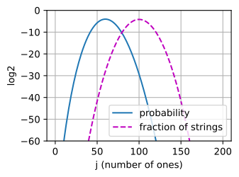
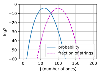
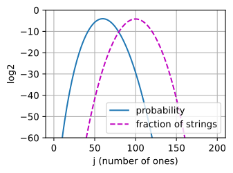
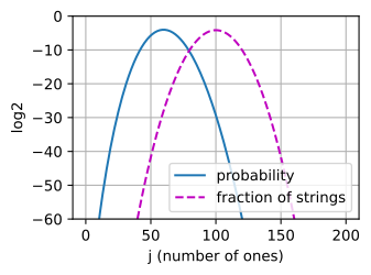
The probability of having \(j\) ones peaks at \(j = 60\), at \(2^{-4.0}\), and the fraction of messages peaks at \(j = 100\), at \(2^{-4.1}\). The single most probable message, at \(j = 0\), has probability \(2^{-103}\) and falls off the chart. The typical messages are therefore neither the most probable messages nor the most numerous ones.
The typical set serves proofs, and it makes a poor coder. Indexing it costs \(189\) bits for every typical message, \(13\) bits above \(nH = 176.3\), plus the flag bit. Arithmetic coding of the same source with the true model averages under \(nH + 2 = 178.3\) bits by Equation 28.2.4. What the typical set shows is that a long message almost surely has the source’s composition, and that about \(2^{nH}\) messages have that composition.
28.2.4 Perplexity
28.2.4.1 Perplexity as a Branching Factor
Language models report one number on held-out text, and it is the quantity this section has been studying. For a text of \(n\) tokens and a model with next-token probabilities \(q(\cdot \mid x_{<i})\), the per-token cross-entropy in nats and its exponential, the perplexity (Jelinek et al. 1977), are
\[ \textrm{CE} = -\frac{1}{n}\sum_{i=1}^n \log q(x_i \mid x_{<i}), \qquad \textrm{PPL} = \exp(\textrm{CE}) = \Big(\prod_{i=1}^n q(x_i \mid x_{<i})\Big)^{-1/n}. \tag{28.2.9}\]
Thus perplexity is the inverse geometric mean of the probabilities the model assigned to the tokens that occurred. A model that is uniformly undecided among \(k\) tokens at every step has \(\textrm{CE} = \ln k\) and \(\textrm{PPL} = k\). A perplexity of \(20\) therefore means that the model is, on average, as uncertain as a uniform choice among \(20\) tokens: it is an effective branching factor. A perfect model of a deterministic sequence has perplexity \(1\). Since \(\textrm{PPL} = b^{\textrm{CE}_b}\) for the cross-entropy \(\textrm{CE}_b\) in any log base \(b\), perplexity is the one quantity of this chapter that does not depend on the unit (Exercise 1).
What perplexity does a model reach on a stream of five tokens to which it assigned probabilities \(0.2, 0.1, 0.4, 0.25, 0.05\), and does the base of the logarithm matter?
q_tok = [0.2, 0.1, 0.4, 0.25, 0.05]   # model prob. of each observed token
nll = [-math.log(q_i) for q_i in q_tok]
mean_nll = sum(nll) / len(nll)        # CE in nats
ce2 = mean_nll / math.log(2)          # the same CE in bits
print(f'per-token NLL (nats): {[round(v, 3) for v in nll]}')
print(f'CE = {mean_nll:.4f} nats, perplexity e^CE = {math.exp(mean_nll):.2f}')
print(f'CE2 = {ce2:.4f} bits, 2^CE2 = {2 ** ce2:.2f}')
per-token NLL (nats): [1.609, 2.303, 0.916, 1.386, 2.996]
CE = 1.8421 nats, perplexity e^CE = 6.31
CE2 = 2.6575 bits, 2^CE2 = 6.31A mean of \(1.84\) nats per token gives a perplexity of \(6.31\): the model is as uncertain as a uniform choice among six or so tokens, and the bits give the same perplexity. The geometric mean punishes confident mistakes. The single token of probability \(0.05\) costs \(3.0\) nats, more than the tokens of probability \(0.4\) and \(0.25\) together. The perplexities reported for the language models of Section 8.3 and Chapter 11 are this number.
28.2.4.2 The Perplexity Floor
How low can perplexity go? For a stationary source the floor is the exponentiated entropy rate, and it holds only in expectation. Here we measure the entropy rate \(H_{\textrm{rate}}\) in nats.
Proposition (perplexity floor). Let the text \(X_1, \ldots, X_n\) come from a stationary source, let \(q\) be any model, and let \(\textrm{CE}_n = -\frac1n \sum_{i=1}^n \log q(X_i \mid X_{<i})\). Then
\[ \mathbb{E}[\textrm{CE}_n] \geq H_{\textrm{rate}}, \qquad \mathbb{E}[\textrm{PPL}_n] = \mathbb{E}\big[e^{\textrm{CE}_n}\big] \geq e^{H_{\textrm{rate}}}. \tag{28.2.10}\]
Proof. Fix a prefix \(x_{<i}\). The expected loss of the model on the next token is a cross-entropy between the source’s conditional distribution \(p(\cdot \mid x_{<i})\) and the model’s, and by Gibbs’ inequality it is at least the entropy of the source’s conditional distribution. Averaging over prefixes gives \(\mathbb{E}[-\log q(X_i \mid X_{<i})] \geq \mathbb{E}[-\log p(X_i \mid X_{<i})]\). The log-probability of a text is the sum of its next-token log-probabilities, \(\log p(x_{1:n}) = \sum_i \log p(x_i \mid x_{<i})\), so summing over \(i\) and dividing by \(n\) gives \(\mathbb{E}[\textrm{CE}_n] \geq \tfrac1n H(X_1, \ldots, X_n) \geq H_{\textrm{rate}}\), the last step by the monotone decrease of the block entropy per symbol. Finally, \(e^x\) is convex, so its average lies above its value at the average (Jensen’s inequality): \(\mathbb{E}[e^{\textrm{CE}_n}] \geq e^{\mathbb{E}[\textrm{CE}_n]} \geq e^{H_{\textrm{rate}}}\). \(\blacksquare\)
Thus no model can be less perplexed, on average, than the source’s own randomness allows. For an ergodic source and the true model, the perplexity of one long text converges to \(e^{H_{\textrm{rate}}}\) as \(n \to \infty\), a fact we grant. The floor does not bound the perplexity of a single short text. A source that emits a with probability \(0.9\) has \(e^H = 1.38\), yet its own true model scores a text of ten symbols below that whenever the text contains no b, which happens with probability \(0.9^{10} = 35\%\) (Exercise 9).
28.2.4.3 Perplexity across Tokenizers
Perplexity is computed per token, so it depends on the tokenizer. A tokenizer with longer tokens makes each prediction harder and the perplexity higher, while the text costs the same number of bits. Two models are comparable by perplexity only under one tokenizer. Across tokenizers, convert to bits per character: a text of \(n_{\textrm{char}}\) characters split into \(n_{\textrm{tok}}\) tokens costs \(n_{\textrm{tok}} \log_2 \textrm{PPL}\) bits, so
\[ \textrm{bpc} = \frac{n_{\textrm{tok}}}{n_{\textrm{char}}}\, \log_2 \textrm{PPL}. \tag{28.2.11}\]
Thus bits per character is the total code length divided by the length of the text, which no tokenizer changes. The same conversion with bytes in place of characters gives bits per byte.
We can now build a prefix code from any distribution and bound its expected length by the entropy. We can code any message to within two bits of its surprisal under any next-symbol model, which makes a language model a lossless compressor. We can compare models by their total description length, and read a perplexity as a branching factor with floor \(e^{H_{\textrm{rate}}}\). Every code here needs a model whose probability for each symbol the encoder and the decoder can both evaluate. Two distributions known only through samples, such as a generator’s samples and the data, give no code to measure. Section 28.3 builds comparisons that work from samples.
28.2.5 Summary
A prefix code is a budget, \(\sum_i 2^{-\ell_i} \leq 1\), and the best lengths for a distribution \(P\) are \(\log_2(1/p_i)\) bits. Every uniquely decodable code averages at least \(H_2(P)\) bits per symbol, and the Shannon code stays below \(H_2(P) + 1\). A code built from a model \(Q\) costs the cross-entropy, with the KL divergence as the excess over the matched code. Arithmetic coding rounds once per message, so any next-symbol model, a language model included, codes a message in its surprisal plus at most two bits, and MDL compares models by the total length of model and data. For a stationary source the entropy rate is the least average length per symbol, and for independent symbols the AEP puts almost all of the probability of length-\(n\) messages on about \(2^{nH}\) typical messages of probability about \(2^{-nH}\) each. Perplexity is the exponentiated per-token cross-entropy, the same number in every log base, at least \(e^{H_{\textrm{rate}}}\) in expectation, and comparable across models only under one tokenizer.
28.2.6 Exercises
Perplexity across tokenizers. Perplexity is computed per token, so it depends on how a text is split into tokens.
- Show that \(b^{\textrm{CE}_b}\) is the same number for every log base \(b\), where \(\textrm{CE}_b\) is the per-token cross-entropy in base-\(b\) units. Two language models are evaluated on the same text of \(10^6\) characters. The tokenizer of model A splits it into \(2.5 \times 10^5\) tokens, and A reaches a per-token perplexity of \(20\). The tokenizer of model B splits it into \(6.7 \times 10^5\) tokens, and B reaches a per-token perplexity of \(8\). Convert both results to bits per character with Equation 28.2.11. Which model predicts the text better?
- Take the entropy rate of the text to be one bit per character, the estimate of Shannon (1951) . By Equation 28.2.10 the expected per-token perplexity is at least \(2^{H}\), where \(H\) is the entropy rate per token in bits. What is the lowest perplexity any model can reach in expectation with the tokenizer of A, and with that of B? How far is each model from its floor?
- Explain in two sentences why the two perplexities cannot be compared directly while the two values of bits per character can.
Huffman codes. Huffman’s algorithm (Huffman 1952) builds a prefix code by repeatedly merging the two least probable symbols into one symbol of their summed probability, and then assigning \(0\) and \(1\) to the two members of each merge.
- Run it on \(P = (0.6, 0.3, 0.1)\) and on \((0.4, 0.3, 0.2, 0.1)\). Report the codeword lengths and the expected length of each code, next to the Shannon code and \(H_2\).
- Prove that Huffman’s code has the smallest expected length of all prefix codes. First show that in an optimal code \(p_i > p_j\) implies \(\ell_i \leq \ell_j\), and that the two longest codewords have the same length and can be taken to be siblings in the tree. Then show that merging the two least probable symbols \(i, j\) reduces the problem by one symbol with \(\mathbb{E}[\ell] = \mathbb{E}[\ell'] + p_i + p_j\), where \(\ell'\) are the lengths of the merged code. Conclude by induction. Hint: exchange two codewords and compare the expected lengths.
- For the source that emits
awith probability \(0.9\), show that every symbol code spends at least one bit per symbol. Then code pairs of symbols as a four-symbol source with Huffman’s algorithm and compute the bits per original symbol. How large is the codebook for blocks of \(n\) symbols, and how does arithmetic coding avoid building it?
McMillan’s theorem. A code is uniquely decodable if every concatenation of codewords parses in only one way.
- Show that the code \(\{0, 01, 011\}\) is uniquely decodable but not prefix-free, and check that it satisfies the Kraft inequality.
- Prove that every uniquely decodable code satisfies the Kraft inequality Equation 28.2.1. Hint: expand \(\big(\sum_i 2^{-\ell_i}\big)^m\) as a sum over all strings of \(m\) codewords of \(2^{-(\textrm{total length})}\), and group the strings by their total length \(L\), where \(m \leq L \leq m \ell_{\max}\). Unique decodability allows at most \(2^L\) strings of total length \(L\), so the sum is at most \(m \ell_{\max}\). Take \(m\)-th roots and let \(m \to \infty\).
- Conclude that restricting to prefix codes costs nothing in expected length.
Where the slack goes. A code with lengths \(\ell_i\) spends \(Z = \sum_i 2^{-\ell_i} \leq 1\) of its budget and implies the distribution \(q_i = 2^{-\ell_i}/Z\), and Equation 28.2.2 writes \(\mathbb{E}[\ell] - H_2(P) = D_{\textrm{KL}}^{(2)}(P\|Q) - \log_2 Z\).
- For the Shannon code of \(P = (0.6, 0.3, 0.1)\), with lengths \(1, 2, 4\), compute \(Z\), \(Q\) and both terms.
- Do the same for Huffman’s lengths \(1, 2, 2\). Which code wastes bits on unspent budget, and which on mismatch?
- Huffman’s code for \(Q = (0.2, 0.5, 0.3)\) has lengths \(2, 1, 2\). Compute its expected length on data from \(P\) and compare it with \(\textrm{CE}_2(P, Q)\). It is smaller. Why does this not contradict the lower bound of Equation 28.2.3?
- For the dyadic source \(P = (\tfrac12, \tfrac14, \tfrac18, \tfrac18)\) and the uniform distribution \(U\) on four symbols, show that \(D_{\textrm{KL}}^{(2)}(P\|U) = D_{\textrm{KL}}^{(2)}(U\|P) = 0.25\) bits. Compute both directions for the running pair \(P, Q\) to show that the symmetry is a coincidence.
[code] Exact arithmetic coding. ● The interval narrowing of Section 28.2.2.1 stores
loandhias floating-point numbers. Draw a message of \(n = 1000\) symbols, each of which isawith probability \(0.9\) andbotherwise.- Run the floating-point narrowing on this message with the model \(q(\texttt{a}) = 0.9\). After how many symbols does
hi - lofirst differ from the product of the probabilities by more than \(0.1\%\), and after how many does it become zero? Relate both answers to the \(53\)-bit significand of a double-precision number. - Repeat the narrowing with exact rationals (
fractions.Fraction). Name a point of the final interval as the text’s cell does, write a decoder that replays the model to recover the message, and compare the code length with the surprisal of the message and with \(n H_2(0.9, 0.1)\). - Encode the same message with the mismatched model \(q(\texttt{a}) = 0.7\). Compare the increase in code length with \(n D_{\textrm{KL}}^{(2)}(P \| Q)\). Why do the two numbers differ for a single message?
- Run the floating-point narrowing on this message with the model \(q(\texttt{a}) = 0.9\). After how many symbols does
[code] Typical and high-probability sets. ● The code of Section 28.2.3.2 declares a binary string of length \(n = 200\) from a Bernoulli source with \(p = 0.3\) typical when its surprisal per symbol lies within \(\delta = 0.1\) bit of the entropy \(H\) in bits. It finds \(2^{188.8}\) typical strings, inside the bounds \(0.989 \cdot 2^{156.3} \leq |A_\delta| \leq 2^{196.3}\) of the AEP proposition and well above \(2^{nH} = 2^{176.3}\).
- Which string is the most probable one? Compute its surprisal per symbol and decide whether it is typical. Why does this string not matter for compression?
- Let \(A\) be the typical set and let \(B\) be any set of strings with \(P(B) \geq 1 - \eta\). Show that \(P(A \cap B) \geq 1 - \eta - P(A^c)\), and conclude that \(|B| \geq \big(1 - \eta - P(A^c)\big)\, 2^{n(H - \delta)}\).
- The smallest set with probability at least \(0.9\) collects strings in order of decreasing probability. Group the strings by their number \(j\) of ones, as the code does, and compute \(\tfrac{1}{n}\log_2\) of the size of this set for \(n = 200\), \(1000\), \(5000\), and \(20000\). Compare it with \(H\) and with \(\tfrac{1}{n}\log_2 |A_\delta|\) at the same \(n\). Which of the two sets grows like \(2^{nH}\), and why does the typical set with a fixed \(\delta\) not?
Adapted from David Tse, EE376A/Stats376A: Information Theory, Homework 2, Problem 6.
Two-part code for a coin. ● A sequence \(\mathcal{D}\) of \(n\) coin flips contains \(j\) heads, and \(\hat\theta = j/n\). Hypothesis \(\mathcal{M}_0\) is the fair coin: it has no parameter to describe, and \(L(\mathcal{D} \mid \mathcal{M}_0) = n \log 2\). Hypothesis \(\mathcal{M}_1\) is a coin with bias \(\theta\). Its encoder sends the point \(\theta_q\) nearest to \(\hat\theta\) on a grid of spacing \(\Delta\) in \((0, 1)\), which costs \(L(\mathcal{M}_1) = \log(1/\Delta)\), and the decoder knows \(n\) and \(\Delta\).
- Use Equation 28.2.3, in nats, to show that \(L(\mathcal{D} \mid \mathcal{M}_1) = n H_b(\hat\theta) + n D_{\textrm{KL}}(\hat\theta \,\|\, \theta_q)\), where the KL divergence is that of the Bernoulli distributions with these parameters. Expand the KL term to second order and show that the total length Equation 28.2.5 of \(\mathcal{M}_1\) exceeds \(n H_b(\hat\theta)\) by at most about \(\log(1/\Delta) + n\Delta^2 / \big(8\hat\theta(1 - \hat\theta)\big)\).
- Which spacing \(\Delta\) minimizes this bound? The decoder must know \(\Delta\) before it decodes \(\theta_q\). Why can the code therefore not use the minimizer? Show that the spacing \(\Delta = 1/\sqrt{n}\), which depends on \(n\) alone, gives an excess of \(\tfrac{1}{2}\log n + O(1)\) whenever \(\hat\theta\) stays bounded away from \(0\) and \(1\).
- Take \(n = 1000\) and the approximation \(L(\mathcal{M}_1) + L(\mathcal{D} \mid \mathcal{M}_1) \approx n H_b(\hat\theta)/\ln 2 + \tfrac{1}{2}\log_2 n\) bits. The text showed that \(\mathcal{M}_1\) wins at \(j = 600\) by \(24\) bits. Which hypothesis wins at \(j = 520\)? Approximately how far from \(n/2\) must \(j\) lie for \(\mathcal{M}_1\) to win, and how many standard deviations \(\sqrt{n}/2\) of \(j\) under the fair coin is that?
Entropy rate of a two-state chain. A chain on \(\{\texttt{a}, \texttt{b}\}\) moves from
atobwith probability \(0.1\) and frombtoawith probability \(0.3\), and it starts from its stationary distribution.- Find the stationary distribution and \(H(X_1)\) in bits.
- Show that \(H(X_n \mid X_{n-1}) = \sum_s \pi_s H_b(r_s)/\ln 2\) bits, where \(\pi\) is the stationary distribution and \(r_s\) is the exit probability of state \(s\), and that the entropy rate equals this value. Compute it.
- Show that \(\tfrac1n H(X_1, \ldots, X_n) = \tfrac1n\big(H(X_1) + (n-1) H_{\textrm{rate}}\big)\) and that it decreases to \(H_{\textrm{rate}}\).
- Consider two limits. With both transition probabilities equal to \(\tfrac12\) the chain is i.i.d. and the rate is \(1\) bit. With both stay probabilities equal to \(\sigma\), the rate tends to \(0\) as \(\sigma \to 1\), while \(H(X_1)\) stays at \(1\) bit. What does \(H(X_1)\) say about how well the chain compresses?
- [code] Simulate \(10^5\) steps of the first chain and code them with the text’s
adaptive_bitsat orders \(0\), \(1\) and \(2\). Which orders reach the rate, and what does the order-\(0\) length converge to?
The perplexity floor.
- Prove Equation 28.2.10, saying where Gibbs’ inequality, the monotone decrease of \(\tfrac1n H(X_1, \ldots, X_n)\) and Jensen’s inequality enter.
- A Bernoulli source emits
awith probability \(0.9\) andbotherwise, and its own true model scores texts of \(n = 10\) symbols. Write \(\textrm{CE}_{10}\) as a function of the number ofb’s and show that \(\textrm{PPL}_{10} < e^{H}\) exactly when the text has nob. What is the probability of that? - A leaderboard reports one perplexity on one held-out set. Explain why Equation 28.2.10 does not bound that number, and why a lower reported perplexity, under the same tokenizer, nevertheless always means a smaller total surprisal of that set, which is its arithmetic code length to within two bits.
[extended] Adaptive context-model compression. ●● The text’s
adaptive_bitsis a complete description length in the sense of Equation 28.2.5, with the cost of learning the model inside it. By Equation 28.2.4, an arithmetic coder driven by its predictions spends at most two bits more. Blier and Ollivier (2018) use such prequential codes to measure the description length of deep networks.- Extend the text’s experiment to \(m = 0, 1, \ldots, 8\). For each \(m\), compare the adaptive code length with the per-character cross-entropy of the order-\(m\) model whose counts are taken from the entire text, and with
zlib. - Explain why the adaptive code length has a minimum over \(m\) while the cross-entropy of the fitted model keeps falling. Which order does MDL select? Which term of Equation 28.2.5 does the cross-entropy of the fitted model leave out?
- Design an adaptive model that combines contexts of several orders, for example by falling back to shorter contexts when a long context has few counts. Report a table of bits per character for every model you tried, together with
zlib, and a paragraph on the design choice that mattered most.
- Extend the text’s experiment to \(m = 0, 1, \ldots, 8\). For each \(m\), compare the adaptive code length with the per-character cross-entropy of the order-\(m\) model whose counts are taken from the entire text, and with