from scipy import integrate37.5 Score-Based Comparisons
A softmax turns ten logits into probabilities by exponentiating them and dividing by their sum, and nobody gives the sum a second thought. Now let a network assign such a number not to ten classes but to every possible input. By convention the sign is reversed: the network returns an energy \(E(\mathbf{x})\), low for plausible images where a logit would be high, and the density is proportional to \(\tilde{q}(\mathbf{x}) = e^{-E(\mathbf{x})}\). The sum becomes an integral over all images, \(Z = \int \tilde{q}(\mathbf{x})\, d\mathbf{x}\), and nobody can compute it. Such an energy-based model can say how plausible an input is, but not how probable.
None of our comparisons applies to it. The likelihood needs the density \(q = \tilde{q}/Z\). The others, by a critic (Section 37.3.4), a kernel or a transport plan (Section 37.4), need samples of the model, and an energy does not hand out samples. Each one has to be produced by a long random walk, many small noisy steps toward lower energy, and every step needs a gradient of the network (Section 38.5.2).
One such gradient is cheap, however, and it is all that we shall ask of the model. The gradient of \(\log \tilde{q}\) with respect to the input, the slope of the log-density, costs one backward pass, and \(Z\) has disappeared from it, because a constant has no slope. This gradient is called the score, and this section compares distributions through scores alone. The mean squared difference of two scores is the objective of score matching, on which diffusion models (Chapter 17) are trained. It has a limit that anyone who trains such a model should know. A slope is local, and it cannot tell how mass is divided between modes that lie far apart. We measure how little it sees.
As before, \(P\) is the data, which we hold as samples, and \(Q\) is the model, which we know through its score \(s_Q\). We ask what a difference of slopes says about two distributions and what it misses, and then how slopes can be compared at all when the data, a finite set of points, have none. Section 38.5.1 builds on these two answers. A third question, how to test a sample against a model that cannot be sampled, can be skipped on a first reading. The section ends with a table of training objectives and advice on choosing among them.
The examples are Gaussians and mixtures of two Gaussians on the line. The helper functions evaluate the log-density of a mixture, with the largest term factored out so that the tails do not underflow (Section 35.8.2), and the KL divergence between two densities on a grid, in nats.
def log_components(x, w, mus, sigmas):
    """log(w_k N(x; mu_k, sigma_k^2)) for every component k; shape (k, len(x))."""
    return (np.log(w)[:, None] - 0.5 * np.log(2 * np.pi * sigmas[:, None] ** 2)
            - (x - mus[:, None]) ** 2 / (2 * sigmas[:, None] ** 2))

def log_mix(x, w, mus, sigmas):
    """Log-density of the mixture sum_k w_k N(mu_k, sigma_k^2), computed stably."""
    c = log_components(x, w, mus, sigmas)
    c_max = c.max(axis=0)
    return c_max + np.log(np.exp(c - c_max).sum(axis=0))

def kl(log_a, log_b, x):
    """D_KL(A||B) by quadrature on the grid x; in nats."""
    return integrate.trapezoid(np.exp(log_a) * (log_a - log_b), x)
37.5.1 The Score and the Fisher Divergence
37.5.1.1 The Score
The score answers one question at every point: in which direction does the density rise, and how steeply? For a distribution \(P\) with a differentiable density \(p\), the score is the gradient of the log-density with respect to the data point:
\[ s_P(\mathbf{x}) = \nabla_{\mathbf{x}} \log p(\mathbf{x}). \tag{37.5.1}\]
(In classical statistics, “score” means the gradient of the log-likelihood with respect to the parameters, as in Section 36.6. Here the gradient is in \(\mathbf{x}\).) For a Gaussian \(\mathcal{N}(\mu, \sigma^2)\) on the line it is
\[ s(x) = -\frac{x - \mu}{\sigma^2}, \]
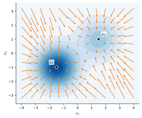
a spring pulling toward the mean with stiffness \(1/\sigma^2\). For a mixture \(p = \sum_k w_k\, p_k\) the chain rule gives \(s(x) = \sum_k r_k(x)\, s_k(x)\) with \(r_k(x) = w_k p_k(x) / p(x)\): each component’s spring, weighted by the posterior probability, or responsibility, that \(x\) came from that component. Near a mode one responsibility is close to \(1\) and the point feels that mode’s spring alone, as Figure 37.5.1 shows. The code is the same formula, with the responsibilities computed from log-densities.
def mix_score(x, w, mus, sigmas):
    """Score of a Gaussian mixture: responsibility-weighted component scores."""
    r = np.exp(log_components(x, w, mus, sigmas) - log_mix(x, w, mus, sigmas))
    return np.sum(r * -(x - mus[:, None]) / sigmas[:, None] ** 2, axis=0)
The score does not depend on a normalizing constant, and that is why we are interested in it. If \(q(\mathbf{x}) = \tilde{q}(\mathbf{x}) / Z\), then
\[ \nabla_{\mathbf{x}} \log q(\mathbf{x}) = \nabla_{\mathbf{x}} \log \tilde{q}(\mathbf{x}) - \nabla_{\mathbf{x}} \log Z = \nabla_{\mathbf{x}} \log \tilde{q}(\mathbf{x}), \]
since \(Z\) does not depend on \(\mathbf{x}\). The unnormalized density \(\tilde{q}(x) = e^{-x^4/4}\), for instance, has the score \(-x^3\), and we never had to find out that \(Z \approx 2.56\).
37.5.1.2 The Fisher Divergence
A comparison built from scores can therefore be applied to an unnormalized model. The natural candidate is the mean squared difference of the two vector fields under the data, the Fisher divergence:
\[ D_{\textrm{F}}(P\|Q) = \frac{1}{2}\, \mathbb{E}_{\mathbf{x} \sim P}\!\left[ \big\| s_P(\mathbf{x}) - s_Q(\mathbf{x}) \big\|^2 \right]. \tag{37.5.2}\]
It is non-negative, and it is a divergence, zero only for \(P = Q\) (Section 37.3.1.1), when both densities are positive on the same connected region. There, equal scores force \(\log p - \log q\) to be constant, and normalization makes the constant zero.
Two Gaussians show how it differs from the KL divergence. With equal variance \(\sigma^2\) and means a distance \(\Delta\) apart, the scores differ by the constant \(\Delta/\sigma^2\) at every \(x\), so
\[ D_{\textrm{F}} = \frac{\Delta^2}{2\sigma^4} \qquad \textrm{whereas} \qquad D_{\textrm{KL}} = \frac{\Delta^2}{2\sigma^2} \]
by the formula for two Gaussians in Section 37.1. At \(\sigma = 1\) the two agree. Measure \(x\) in units half as large, and \(\Delta\) and \(\sigma\) both double: the KL divergence stays where it was, and the Fisher divergence falls to a quarter. It is measured in units of \(1/x^2\), as a squared slope must be, and not in nats. Its size therefore depends on the units of the data, and a score-matching loss on one data set cannot be compared with the loss on another, or with a budget in nats. Exercise 1a treats unequal variances, and Exercise 2 a general change of variables.
37.5.1.3 Mixing Weights of Distant Modes
The average in Equation 37.5.2 runs over the data, and what it averages is a difference of slopes. For data with several modes the two facts combine badly. Take two mixtures with the same components and swapped weights,
\[ P_w = w\,\mathcal{N}(-m, 1) + (1 - w)\,\mathcal{N}(m, 1), \qquad w = 0.7 \textrm{ against } w = 0.3. \]
As distributions the two are far apart. Once the modes are well separated, their KL divergence is that of the weight vectors \((0.7, 0.3)\) and \((0.3, 0.7)\), which is \(0.7 \log\tfrac{7}{3} + 0.3 \log\tfrac{3}{7} = 0.339\) nats, whatever \(m\) is.
The scores hardly differ. Near each mode the responsibility of that mode is close to \(1\) in both mixtures, so both scores are that mode’s spring. Written out (Exercise 3b derives it), the score of \(P_w\) is
\[ s_w(x) = -x + m \tanh(m x - c_w), \qquad c_w = \tfrac{1}{2} \log\frac{w}{1 - w}. \]
This is the spring \(-(x + m)\) far to the left, the spring \(-(x - m)\) far to the right, and a hand-over between them around \(x = c_w/m\). The weight enters through the place of the hand-over and through nothing else. At \(m = 5\) the hand-over sits at \(x = 0.085\) for \(w = 0.7\) and at \(x = -0.085\) for \(w = 0.3\), in the valley between the modes, where the density is \(e^{-m^2/2}/\sqrt{2\pi}\), about \(1.5 \times 10^{-6}\). The data almost never visit the one place where the two scores disagree. We compute both divergences by quadrature as the modes move apart, and expect the Fisher divergence to fall roughly like \(e^{-m^2/2}\).
xs = np.linspace(-14.0, 14.0, 14001)
w_a, w_b, unit = np.array([0.7, 0.3]), np.array([0.3, 0.7]), np.ones(2)
for m in (1.0, 3.0, 5.0):
    mus_m = np.array([-m, m])
    log_a, log_b = log_mix(xs, w_a, mus_m, unit), log_mix(xs, w_b, mus_m, unit)
    score_gap = mix_score(xs, w_a, mus_m, unit) - mix_score(xs, w_b, mus_m, unit)
    fisher = 0.5 * integrate.trapezoid(np.exp(log_a) * score_gap ** 2, xs)
    print(f'm = {m:.0f}: KL = {kl(log_a, log_b, xs):.3f} nats, '
          f'Fisher = {fisher:.1e}')
m = 1: KL = 0.184 nats, Fisher = 1.1e-01
m = 3: KL = 0.337 nats, Fisher = 7.1e-03
m = 5: KL = 0.339 nats, Fisher = 4.0e-06The KL divergence settles at \(0.339\) nats, and the Fisher divergence falls by more than four orders of magnitude, from about \(0.1\) to about \(4 \times 10^{-6}\). At \(m = 5\) it is of the size of \(e^{-m^2/2} = e^{-12.5} \approx 4 \times 10^{-6}\), as the empty valley led us to expect. A loss built from scores cannot see how mass is divided between distant modes. The word “connected” above was a warning: on two separate regions, equal scores allow \(\log p - \log q\) a constant of its own on each (Exercise 4). A model fitted to such data by minimizing the Fisher divergence can give both modes the right place and the right shape and still hold \(30\%\) of its mass where the data hold \(70\%\) (Wenliang and Kanagawa 2020).
Noise fills the valley. Add independent Gaussian noise of standard deviation \(2\) to both mixtures, and the variance of every mode grows from \(1\) to \(5\). The modes, ten standard deviations apart before, are now \(4.5\) apart, and the density in the valley rises from \(1.5 \times 10^{-6}\) to about \(0.015\). The data now visit the place where the two scores disagree (Exercise 3c measures what is gained). This is one reason why diffusion models perturb the data with noise at many scales before they match scores. Section 17.1 measures the same blind spot on trained networks.
37.5.2 Stein’s Identity
The Fisher divergence has a second defect, which stands in the way of any use at all: it contains \(s_P\), the score of the data, and data come as samples. A finite set of points has no slope. To see where \(s_P\) enters, we expand the square. On the line,
\[ D_{\textrm{F}}(P\|Q) = \tfrac{1}{2}\, \mathbb{E}_P\big[s_P^2\big] - \mathbb{E}_P\big[s_P\, s_Q\big] + \tfrac{1}{2}\, \mathbb{E}_P\big[s_Q^2\big]. \tag{37.5.3}\]
The last term is an average over the data of a function that the model supplies, and a sample estimates it. The first does not depend on the model, so it plays no part when models are fitted or ranked. The obstacle is the cross term in the middle, where the unknown score of the data multiplies the score of the model. An identity that every smooth density satisfies with its own score removes it. We state it for one density on the line and then use it twice: for the data, to remove the cross term, and for the model, to test a sample.
Proposition (Stein’s identity). Let \(p > 0\) be a differentiable density on \(\mathbb{R}\) with score \(s = (\log p)'\), and let \(g\) be differentiable with \(g(x)\, p(x) \to 0\) as \(x \to \pm\infty\), \(\mathbb{E}_p|g'| < \infty\) and \(\mathbb{E}_p|g\, s| < \infty\). Then
\[ \mathbb{E}_{x \sim p}\big[ g'(x) + g(x)\, s(x) \big] = 0. \tag{37.5.4}\]
Proof. The score is \(s = p'/p\), so \(p' = s\, p\). One integration by parts (Section 34.6.2.3) gives
\[ \int g'\, p\, dx = \big[ g\, p \big]_{-\infty}^{\infty} - \int g\, p'\, dx = -\int g\, s\, p\, dx, \]
where the boundary term vanishes and both integrals converge by the conditions on \(g\). \(\blacksquare\)
For the standard normal density the score is \(-x\) and the identity reads \(\mathbb{E}[g'(X)] = \mathbb{E}[X g(X)]\). With \(g(x) = x\) it says \(\mathbb{E}[X^2] = 1\). This case is Stein’s lemma for the normal distribution (Stein 1981), and the form for a general density is in (Stein 1986). The identity turns knowledge of a slope into statements about averages, and averages are what samples estimate.
37.5.2.1 Score Matching
Suppose that the data distribution \(P\) has a smooth density, even though we see only samples of it. Then the identity holds for the data, with \(s = s_P\), and we may take the model’s score as the test function, \(g = s_Q\). It reads \(\mathbb{E}_P[s_Q' + s_Q\, s_P] = 0\). The cross term of Equation 37.5.3 is therefore \(-\mathbb{E}_P[s_Q']\), an average that no longer contains \(s_P\), and
\[ D_{\textrm{F}}(P\|Q) = \mathbb{E}_{x \sim P}\Big[ \tfrac{1}{2}\, s_Q(x)^2 + s_Q'(x) \Big] + \tfrac{1}{2}\, \mathbb{E}_P\big[s_P^2\big]. \tag{37.5.5}\]
The derivative has moved from the data, which have none, to the model. The last term is the same for every model, and the rest is an average over the data of quantities that the model supplies: it can be estimated from a sample and minimized, with no \(Z\) and no \(s_P\). This is score matching. Hyvärinen (2005) devised it for models without a normalizing constant and fitted a model of natural image patches with it.
The quartic of Section 37.5.1 shows what has been gained. Give it a parameter, \(\tilde{q}_\theta(x) = e^{-\theta x^4/4}\), so that \(s_Q(x) = -\theta x^3\) and \(s_Q'(x) = -3\theta x^2\). With a bar for an average over the data, the part of Equation 37.5.5 that depends on the model is estimated by
\[ \overline{\tfrac{1}{2}\, s_Q^2 + s_Q'} = \tfrac{1}{2}\, \theta^2\, \overline{x^6} - 3\, \theta\, \overline{x^2}, \qquad \textrm{which is smallest at} \qquad \hat\theta = \frac{3\, \overline{x^2}}{\overline{x^6}}. \]
Two moments of the sample fit the model, and nobody had to integrate \(e^{-\theta x^4/4}\). Maximum likelihood needs \(Z(\theta)\) and arrives at a different function of the data (Exercise 6). For a Gaussian model the two fits coincide (Exercise 5).
On the line, \(s_Q'\) is one more derivative. In \(\mathbb{R}^n\) it becomes a sum of \(n\) second derivatives, one for each coordinate, and the single backward pass that gave the score turns into \(n\) of them, far too many for an image. Section 38.5.1 carries the argument to \(\mathbb{R}^n\), shows how noise added to the data avoids these derivatives, and derives the training loss of diffusion models from the result.
37.5.2.2 A Test for Samples
The identity can also test a sample against a model. Stated for the model, it says that for every \(g\) that meets the conditions of the proposition the function \(g' + g\, s_Q\) averages to zero under \(Q\). The map that takes \(g\) to \(g' + g\, s_Q\) is called the Stein operator of the model. If the average of \(g' + g\, s_Q\) over a sample is far from zero for some \(g\), the sample did not come from \(Q\). The check needs the model’s score at the sample points and nothing else, neither \(Z\) nor samples of the model.
How much can one test function detect? Let the model be \(Q = \mathcal{N}(0, 1)\), so that the function to average is \(g'(x) - x\, g(x)\). For \(g = 1\) this is \(-x\), and the test checks the mean of the sample. For \(g(x) = x\) it is \(1 - x^2\), and the test checks the second moment against \(1\). As a third test function we take \(g(x) = \sin x\), which has no such simple reading. The cell draws \(200{,}000\) points from the model itself, from \(\mathcal{N}(0.5, 1)\), which is shifted, and from \(\mathcal{N}(0, 4)\), which is twice as wide, and prints every average with its standard error. From the two moments we expect \(-0.5\) and \(1 - 1.25 = -0.25\) on the shifted sample, and \(0\) and \(1 - 4 = -3\) on the wide one.
rng = np.random.default_rng()
n = 200_000
# Stein operator of the model Q = N(0, 1), whose score is -x:  g'(x) - x g(x)
tests = [('g = 1', np.ones_like, np.zeros_like),
         ('g = x', lambda t: t, np.ones_like),
         ('g = sin x', np.sin, np.cos)]
samples = [('N(0, 1)', rng.normal(0.0, 1.0, n)),
           ('N(0.5, 1)', rng.normal(0.5, 1.0, n)),
           ('N(0, 4)', rng.normal(0.0, 2.0, n))]
print(f'{"sample":10s}' + ''.join(f'{name:>18s}' for name, _, _ in tests))
for s_name, x in samples:
    vals = [g_prime(x) - x * g(x) for _, g, g_prime in tests]
    print(f'{s_name:10s}' + ''.join(f'{v.mean():+10.3f} ± {v.std() / np.sqrt(n):.3f}'
for v in vals))sample g = 1 g = x g = sin x
N(0, 1) -0.001 ± 0.002 -0.002 ± 0.003 -0.001 ± 0.002
N(0.5, 1) -0.503 ± 0.002 -0.249 ± 0.004 -0.145 ± 0.002
N(0, 4) +0.002 ± 0.004 -3.006 ± 0.013 -0.410 ± 0.003sample g = 1 g = x g = sin x
N(0, 1) -0.002 ± 0.002 +0.001 ± 0.003 +0.003 ± 0.002
N(0.5, 1) -0.501 ± 0.002 -0.250 ± 0.004 -0.146 ± 0.002
N(0, 4) +0.002 ± 0.004 -3.008 ± 0.013 -0.410 ± 0.003sample g = 1 g = x g = sin x
N(0, 1) -0.000 ± 0.002 -0.001 ± 0.003 +0.000 ± 0.002
N(0.5, 1) -0.501 ± 0.002 -0.253 ± 0.004 -0.147 ± 0.002
N(0, 4) -0.002 ± 0.004 -3.005 ± 0.013 -0.404 ± 0.003sample g = 1 g = x g = sin x
N(0, 1) +0.001 ± 0.002 +0.005 ± 0.003 +0.004 ± 0.002
N(0.5, 1) -0.499 ± 0.002 -0.245 ± 0.004 -0.145 ± 0.002
N(0, 4) -0.004 ± 0.004 -3.008 ± 0.013 -0.402 ± 0.003On the model’s own sample no average is further from zero than a few of its standard errors. All three test functions catch the shifted sample, at about \(-0.50\), \(-0.25\) and \(-0.15\). The wide sample is another matter. Its mean is zero, so \(g = 1\) reports no more than a hundredth or so, nothing like the \(-0.5\) of the shift, although a sample with four times the model’s variance is hardly a subtle violation. Only \(g = x\), at about \(-3\), and \(\sin x\), at about \(-0.4\), notice it. A test function checks one property of the sample, and a sample can be wrong in a property that the function does not check.
Why does \(g = 1\) see the shift and miss the width? A sample from a distribution \(P\) with a smooth density obeys the identity of \(P\), \(\mathbb{E}_P[g'] = -\mathbb{E}_P[g\, s_P]\), and therefore
\[ \mathbb{E}_P\big[ g' + g\, s_Q \big] = \mathbb{E}_P\big[ (s_Q - s_P)\, g \big]. \tag{37.5.6}\]
The average is the difference of the two scores, weighted by \(g\). For the shifted sample the difference is the constant \(-x + (x - 0.5) = -0.5\), and \(g = 1\) picks it up in full. For the wide sample it is \(-x + x/4 = -\tfrac{3}{4}x\). This is an odd function, and a distribution that is symmetric about zero averages it to zero when the weight is \(g = 1\). No single test function is correlated with every possible difference of scores.
37.5.3 The Kernel Stein Discrepancy
One test function checks one property, so we use many at once: all functions in the unit ball of a feature space, and among them the one whose average is largest. Section 37.4.1 did the same for the difference of two means and found a closed form, the maximum mean discrepancy (MMD). There is one here as well, which is rather remarkable. A supremum over infinitely many test functions reduces to kernel evaluations on pairs of data points.
Write \(\mathcal{A}_Q\) for the Stein operator of the model \(Q\), \((\mathcal{A}_Q g)(x) = g'(x) + s_Q(x)\, g(x)\), so that Stein’s identity says \(\mathbb{E}_Q[\mathcal{A}_Q g] = 0\), and measure the data distribution \(P\) by \(\sup_g \mathbb{E}_P[\mathcal{A}_Q g]\), the largest amount by which the data violate the identity of the model.
For \(g(x) = \langle \mathbf{w}, \boldsymbol{\varphi}(x) \rangle\) with a feature vector \(\boldsymbol{\varphi}\) and \(\|\mathbf{w}\| \leq 1\), the operator acts on the features: \((\mathcal{A}_Q g)(x) = \langle \mathbf{w}, \boldsymbol{\psi}(x) \rangle\) with \(\boldsymbol{\psi} = \boldsymbol{\varphi}' + s_Q\, \boldsymbol{\varphi}\). By the Cauchy–Schwarz inequality the supremum of \(\langle \mathbf{w}, \mathbb{E}_P[\boldsymbol{\psi}] \rangle\) over the ball is \(\big\| \mathbb{E}_P[\boldsymbol{\psi}] \big\|\), and the square of this norm is \(\mathbb{E}\langle \boldsymbol{\psi}(x), \boldsymbol{\psi}(x') \rangle\) for independent draws \(x, x'\) from \(P\). Multiplying out leaves four inner products of features, and each is the kernel \(k(x, x') = \langle \boldsymbol{\varphi}(x), \boldsymbol{\varphi}(x') \rangle\) or one of its derivatives:
\[ \langle \boldsymbol{\varphi}'(x), \boldsymbol{\varphi}(x') \rangle = \partial_x k, \qquad \langle \boldsymbol{\varphi}(x), \boldsymbol{\varphi}'(x') \rangle = \partial_{x'} k, \qquad \langle \boldsymbol{\varphi}'(x), \boldsymbol{\varphi}'(x') \rangle = \partial_x \partial_{x'} k. \]
Their sum, with the scores as coefficients, is the Stein kernel of \(Q\),
\[ k_Q(x, x') = s_Q(x)\, s_Q(x')\, k(x, x') + s_Q(x)\, \partial_{x'} k(x, x') + \partial_x k(x, x')\, s_Q(x') + \partial_x \partial_{x'} k(x, x'), \tag{37.5.7}\]
and the squared kernel Stein discrepancy (KSD) is its average over two independent draws from the data:
\[ \mathrm{KSD}^2(P, Q) = \mathbb{E}_{x, x' \sim P}\big[ k_Q(x, x') \big]. \tag{37.5.8}\]
The average is taken under the data alone. A sample \(x_1, \ldots, x_N\) from \(P\) therefore gives the unbiased estimator
\[ \widehat{\mathrm{KSD}}^2 = \frac{1}{N(N-1)} \sum_{i \neq j} k_Q(x_i, x_j), \]
the same average over pairs without self-pairs as the MMD estimator. Statisticians call such an average a U-statistic, which is where the name ksd2_ustat in the code below comes from.
To see what the KSD measures, we apply Equation 37.5.6 to each feature. It gives \(\mathbb{E}_P[\boldsymbol{\psi}] = \mathbb{E}_P[(s_Q - s_P)\, \boldsymbol{\varphi}]\), and squaring the norm as before,
\[ \mathrm{KSD}^2(P, Q) = \mathbb{E}_{x, x' \sim P}\big[ (s_Q - s_P)(x)\, k(x, x')\, (s_Q - s_P)(x') \big]. \tag{37.5.9}\]
The KSD is a kernel-smoothed relative of the Fisher divergence \(D_{\textrm{F}}(P\|Q)\): the same difference of scores under the same data distribution, multiplied across pairs of points with weight \(k\) where the Fisher divergence squares it at each point. The blind spot comes along, and it is deeper. On the two mixtures of Section 37.5.1 both points of a pair must now fall into the valley where the scores differ, and \(\mathrm{KSD}^2\) decays roughly like \(e^{-m^2}\), the square of the rate of the Fisher divergence (Exercise 3e).
Where both scores are known, Equation 37.5.9 predicts the value. Let the data be \(P = \mathcal{N}(0, 1)\) and take three models. Against the correct model \(\mathcal{N}(0, 1)\) the difference of scores vanishes and \(\mathrm{KSD}^2 = 0\). Against the shifted model \(\mathcal{N}(1, 1)\) the difference is \(-(x - 1) - (-x) = 1\) at every point, so \(\mathrm{KSD}^2 = \mathbb{E}[k(X, X')]\). For the RBF kernel \(k(x, x') = e^{-(x - x')^2/(2\ell^2)}\) with length scale \(\ell\) this is the Gaussian integral of Section 37.4.1: the difference \(X - X'\) has the distribution \(\mathcal{N}(0, 2)\), and the average of the kernel over it is \((1 + 2/\ell^2)^{-1/2}\). At \(\ell = 1\) we obtain \(\mathrm{KSD}^2 = 1/\sqrt{3} \approx 0.577\).
The third model is of the kind that this section is about: the quartic \(\tilde{q}(x) = e^{-x^4/4}\) of Section 37.5.1, which we know only up to its constant. Its score is \(-x^3\), the difference of scores is \(x - x^3\), and the double integral in Equation 37.5.9 has no such short form. The function ksd2_population in the cell evaluates it on a grid. It can do so because we, unlike the test, know the density of the data.
For the RBF kernel on the line the derivatives in Equation 37.5.7 are \(\partial_{x'} k = \frac{x-x'}{\ell^2}\, k\), \(\partial_x k = -\frac{x-x'}{\ell^2}\, k\) and \(\partial_x \partial_{x'} k = \big( \frac{1}{\ell^2} - \frac{(x-x')^2}{\ell^4} \big)\, k\). In the code, dk_dy is the derivative in the second argument and kappa the matrix of all \(k_Q(x_i, x_j)\). We test one sample of \(2{,}000\) points from \(\mathcal{N}(0, 1)\) against the three models. The function ksd2_ustat receives each model as a score function and as nothing else.
def ksd2_ustat(x, score, ell=1.0):
    """U-statistic KSD^2 with the RBF kernel exp(-(a-b)^2 / (2 ell^2))."""
    d = x[:, None] - x[None, :]
    k = np.exp(-d ** 2 / (2 * ell ** 2))
    dk_dx = -d / ell ** 2 * k
    dk_dy = d / ell ** 2 * k
    d2k = (1 / ell ** 2 - d ** 2 / ell ** 4) * k
    s = score(x)
    kappa = (s[:, None] * s[None, :] * k + s[:, None] * dk_dy
             + dk_dx * s[None, :] + d2k)
    n = len(x)
    return (kappa.sum() - np.trace(kappa)) / (n * (n - 1))

def ksd2_population(score, ell=1.0):
    """KSD^2 of the data P = N(0, 1) against a model with this score, from
    the score difference s_Q - s_P weighted by the kernel, by quadrature."""
    t = np.linspace(-10.0, 10.0, 2001)
    h = np.exp(-t ** 2 / 2) / np.sqrt(2 * np.pi) * (score(t) + t)
    k = np.exp(-(t[:, None] - t[None, :]) ** 2 / (2 * ell ** 2))
    return h @ k @ h * (t[1] - t[0]) ** 2

x_p = rng.standard_normal(2000)          # the data sample, P = N(0, 1)
for name, s in [('true model  N(0,1)', lambda t: -t),
                ('wrong model N(1,1)', lambda t: -(t - 1)),
                ('quartic exp(-x^4/4)', lambda t: -t ** 3)]:
    print(f'KSD^2 vs the {name:19s}: {ksd2_ustat(x_p, s):+.4f}  '
f'(population {ksd2_population(s):.4f})')KSD^2 vs the true model N(0,1) : +0.0010 (population 0.0000)
KSD^2 vs the wrong model N(1,1) : +0.5274 (population 0.5774)
KSD^2 vs the quartic exp(-x^4/4): +0.2835 (population 0.3208)KSD^2 vs the true model N(0,1) : -0.0008 (population 0.0000)
KSD^2 vs the wrong model N(1,1) : +0.5869 (population 0.5774)
KSD^2 vs the quartic exp(-x^4/4): +0.2893 (population 0.3208)KSD^2 vs the true model N(0,1) : +0.0015 (population 0.0000)
KSD^2 vs the wrong model N(1,1) : +0.5681 (population 0.5774)
KSD^2 vs the quartic exp(-x^4/4): +0.4494 (population 0.3208)KSD^2 vs the true model N(0,1) : -0.0004 (population 0.0000)
KSD^2 vs the wrong model N(1,1) : +0.6155 (population 0.5774)
KSD^2 vs the quartic exp(-x^4/4): +0.2739 (population 0.3208)Against the correct model the estimate is within a few thousandths of zero and may be slightly negative, as an unbiased estimate of zero must sometimes be. Against the shifted model, in the second line, it lands close to the predicted \(1/\sqrt{3} \approx 0.58\), within about \(0.1\). Against the quartic it is a few tenths, far from zero. The population value is \(0.32\) here, and a single sample can miss it by \(0.1\) and more, because the score \(-x^3\) is large at the few points far from the origin and these dominate the average.
Between the three lines of output only the score function changed. The sample is the same, no model was sampled, and the normalizing constant of the quartic, \(Z \approx 2.56\), appears nowhere in the code.
With the RBF kernel a value of zero can be trusted. For data with a smooth density, and under mild conditions on the two scores, \(\mathrm{KSD}^2(P, Q) = 0\) if and only if \(P = Q\) (Liu et al. 2016; Chwialkowski et al. 2016). The two mixtures are a reminder that the value can nevertheless be tiny for distributions that are far apart.
In \(\mathbb{R}^n\) only the notation changes: \(g\) is a vector field, the operator is \(s_Q^\top g + \nabla \cdot g\), the products in Equation 37.5.7 become inner products of vectors, and the last term becomes \(\sum_i \partial_{x_i} \partial_{x'_i} k\). The KSD serves as a goodness-of-fit test for unnormalized models and as a check on the output of a sampler. Applied to the kernel itself, the Stein operator also gives a direction in which to move the points of a sample toward the model, a method called Stein variational gradient descent (Liu and Wang 2016). No training objective in this book uses the KSD.
37.5.4 Training Objectives and Their Divergences
The two sections before this one produced three families of comparisons, and this one has added two comparisons of scores. Figure 37.5.2 places the families and the members they share. It does not draw the Fisher divergence, which belongs to none of the three. Nor does it draw the KSD, which has the form of the second family, a largest difference of averages over a class of test functions, but with a class that is built from the model’s score and changes with the model.
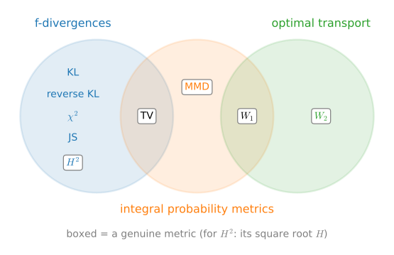
Table 37.5.1 lists the objectives that are built on these comparisons. Each row names an objective, what it needs from the model and the data, and the divergence that it minimizes when its averages are taken over the whole distributions and, for the adversarial objectives, the critic is the best possible. A critic, as in Section 37.3.4, is a function trained on the two samples, in practice a second network. The fourth column returns to the test case with which Section 37.3 began, the data at a single point, \(P = \delta_0\), and the model’s samples at a point a distance \(d\) away, \(Q = \delta_d\). A comparison that does not change with \(d\) gives such a model no gradient toward the data.
| What the objective needs | Objective | Divergence | Two point masses \(d\) apart | Treated in |
|---|---|---|---|---|
| model density at data points | maximum likelihood (autoregressive models, flows) | forward KL | \(\infty\) | Section 37.3.2 |
| samples of both, through a critic | original GAN | Jensen–Shannon | \(\log 2\), constant | Section 37.3.4 |
| samples of both, through a critic | f-GAN | the chosen \(D_f\) | \(f(0) + f'(\infty)\), constant | Section 37.3.4 |
| samples of both, no critic for a fixed kernel | moment matching, two-sample tests | MMD | \(\textrm{MMD}^2 = 2 - 2e^{-d^2/(2\ell^2)}\), flat beyond a few \(\ell\) | Section 37.4.1 |
| samples of both, a 1-Lipschitz critic | WGAN | \(W_1\) | \(d\) | Section 37.4.2 |
| model samples, the model’s density at them, the unnormalized target | variational inference, VAE posterior | reverse KL | \(\infty\) | Section 37.3.2 |
| model score, data samples | score matching, diffusion models | Fisher | undefined (a point mass has no score) | Section 37.5.1 |
| model score, data samples | goodness-of-fit tests, sampler quality | KSD | undefined (a point mass has no score) | Section 37.5.3 |
Read from the top, the table is advice, because its rows are ordered by what a model can supply. A model whose density can be evaluated, and is positive wherever data may fall, should be trained by maximum likelihood: forward KL needs nothing but the data, its sample average is unbiased, and it leaves no mode of the data uncovered. A model that only produces samples has three choices. A critic trained as in a GAN is the usual one for images (Section 16.1), where nobody knows in advance which features tell the model’s samples from the data, and the critic learns them. Its estimate of the divergence is biased low and goes flat when the samples are far from the data (Section 37.3.4). A 1-Lipschitz critic is the choice for a model that starts far away, because \(W_1\) keeps its slope at every distance (Section 16.2 trains with both kinds). A fixed kernel needs no second network, and the error of its estimate is of order \(N^{-1/2}\) in any dimension (Section 37.4.1). It suits two-sample tests and the evaluation of samples, and it loses its gradient beyond a few length scales.
The last three rows are for the cases in which a normalizing constant is missing. When it is the target that is known only up to its constant, and the model can be sampled and has a density, as in variational inference, reverse KL applies, at the risk of settling on one mode. And a model known only through its score calls for the Fisher divergence, which leaves the weights of distant modes undetermined unless noise is added, as diffusion models do (Section 17.1).
The table says which comparison an objective makes. It does not say how well that comparison can be made from data. Every sample-based number of these three sections, the critic bound, \(\textrm{MMD}^2\) and \(\mathrm{KSD}^2\), is an estimate with an error, and the critic bound is biased low besides. The next two sections turn from two distributions to two variables. Section 37.6 uses the KL divergence to measure how much one variable tells about another, and Section 37.7 asks how much of it a sample of \(n\) pairs can certify.
37.5.5 Summary
A model that is known only up to its normalizing constant can still be compared with data through its score, the gradient of the log-density with respect to the input, from which the constant drops out. The Fisher divergence is the mean squared difference of two scores under the data, and Stein’s identity, one integration by parts, removes the unknown score of the data from it. Scores are local: between two mixtures that differ only in the weights of two modes ten standard deviations apart, the Fisher divergence is \(4 \times 10^{-6}\) while the KL divergence is \(0.339\) nats. The kernel Stein discrepancy uses the same identity to test a sample against a model through the model’s score alone. Which comparison to train on is decided by what the model can supply: a density, samples, or a score.
37.5.6 Exercises
- Fisher divergence and Stein moments. The score of \(\mathcal{N}(\mu, \sigma^2)\) is \(-(x - \mu)/\sigma^2\).
- Compute the Fisher divergence Equation 37.5.2 between \(\mathcal{N}(\mu_1, \sigma_1^2)\) and \(\mathcal{N}(\mu_2, \sigma_2^2)\) in closed form, and check that it reduces to \((\mu_1 - \mu_2)^2 / (2\sigma^4)\) for equal variances. Is the Fisher divergence symmetric?
- Apply Stein’s identity Equation 37.5.4 for \(\mathcal{N}(0, 1)\) to \(g(x) = x^k\), derive the recursion \(\mathbb{E}[X^{k+1}] = k\, \mathbb{E}[X^{k-1}]\), and compute \(\mathbb{E}[X^4]\) and \(\mathbb{E}[X^6]\). What does \(g(x) = 1\) give for a general density that satisfies the conditions of the identity?
- Let the data distribution \(P\) on \(\mathbb{R}\) have finite moments of all orders, and let \(\mathbb{E}_P[g'(X) - X g(X)] = 0\) for every polynomial \(g\). Explain why \(P = \mathcal{N}(0, 1)\), using that the normal distribution is determined by its moments. Then let \(P(X = 1) = P(X = -1) = \tfrac{1}{2}\), and show that it satisfies the identity for every polynomial \(g\) of degree at most \(2\) but not for \(g(x) = x^3\). What does this imply for a goodness-of-fit test that checks the identity only on polynomials up to a fixed degree?
- Units and changes of variables. Let \(a > 0\), and write \(P_a\) and \(Q_a\) for the distributions of \(aX\) when \(X\) is drawn from \(P\) and from \(Q\).
- Show that \(D_{\textrm{KL}}(P_a\|Q_a) = D_{\textrm{KL}}(P\|Q)\) and \(D_{\textrm{F}}(P_a\|Q_a) = D_{\textrm{F}}(P\|Q)/a^2\). A set of images is stored once with pixel values between \(0\) and \(255\) and once with values between \(0\) and \(1\). By what factor does the Fisher divergence between the data and a model differ in the two units?
- Replace the scaling by a smooth increasing map \(y = \phi(x)\) of the line. Show that the two scores at \(y\) differ by \(\big(s_P(x) - s_Q(x)\big)/\phi'(x)\), although each of them gains a term in \(\phi''\). Conclude that the Fisher divergence becomes \(\tfrac{1}{2}\, \mathbb{E}_P\big[(s_P - s_Q)^2 / \phi'^2\big]\), while the KL divergence does not change.
- A change of variables can therefore make a Fisher divergence that is not zero as large or as small as we please. For the two mixtures of the text, where on the line would \(\phi\) have to be nearly flat to make the difference of the weights visible?
- [code] Score blindness to mixing weights. ● Let \(P_w = w\, \mathcal{N}(-m, 1) + (1 - w)\, \mathcal{N}(m, 1)\).
- The text computes \(D_{\textrm{F}}(P_{0.7}\|P_{0.3})\) and \(D_{\textrm{KL}}(P_{0.7}\|P_{0.3})\) for \(m \in \{1, 3, 5\}\). Extend the computation to \(m \in \{1, \ldots, 6\}\). Show that the KL divergence tends to \(0.4 \log\tfrac{7}{3}\), the value \(0.339\) of the text, and find the rate at which the Fisher divergence decays by fitting \(\log D_{\textrm{F}}\) against \(m^2\).
- Derive the score \(s_w(x) = -x + m \tanh(m x - c_w)\) of the text from the responsibilities. Show that \(s_{0.7}\) and \(s_{0.3}\) differ most at \(x = 0\), by \(0.8\,m\), and substitute \(u = m x\) in the Fisher divergence to show that it behaves like \(C\, m\, e^{-m^2/2}\) for large \(m\), with a constant \(C\) that depends only on the weights. Compare with the rate you fitted in (a). What does the result imply for the mixing weights of a model fitted by score matching (Wenliang and Kanagawa 2020)?
- Add independent \(\mathcal{N}(0, \sigma^2)\) noise to samples of both mixtures, so that each component becomes \(\mathcal{N}(\pm m, 1 + \sigma^2)\). Repeat (a) at \(m = 5\) for \(\sigma \in \{0, 0.5, 1, 2\}\). How does the noise change the two divergences? Heavy noise shows the weights and blurs the shape of each mode, and light noise does the opposite. Why would a model that matches scores at several noise levels recover both (Song and Ermon 2019)?
- Write \(P_t\) and \(Q_t\) for two distributions after independent \(\mathcal{N}(0, t)\) noise has been added to both. For two Gaussians of equal variance \(\sigma^2\), which the noise raises to \(\sigma^2 + t\), check from the two closed forms of the text that \(\frac{d}{dt} D_{\textrm{KL}}(P_t\|Q_t) = -D_{\textrm{F}}(P_t\|Q_t)\). The identity holds for every pair of smooth densities. Confirm it by a finite difference for the two mixtures at \(m = 5\) and \(t \in \{1, 4, 9\}\), and conclude that \(D_{\textrm{KL}}(P\|Q) = \int_0^\infty D_{\textrm{F}}(P_t\|Q_t)\, dt\). At which noise level is the Fisher divergence largest? What does the integral say about matching scores at one noise level against matching them at all levels (Song et al. 2021)?
- The kernel Stein discrepancy has the same blind spot. Evaluate Equation 37.5.9 for the two mixtures by quadrature on a grid, with the RBF kernel at \(\ell = 1\) and \(m \in \{1, 3, 5\}\), and compare with the Fisher divergences of the text (at \(m = 5\) you should find about \(10^{-11}\)). The function
ksd2_populationof the text is the pattern; it is written for the data \(\mathcal{N}(0, 1)\), and here the data are \(P_{0.7}\). Where must both points of a pair fall to contribute, and how wide is that region compared with \(\ell\)? Conclude that \(\mathrm{KSD}^2\) decays like \(e^{-m^2}\). Would a smaller length scale help?
- Two separate regions. Let \(p_0(x) = 30\, x^2 (1 - x)^2\) for \(0 < x < 1\) and \(p_0(x) = 0\) elsewhere, and let \(P_w\) have the density \(w\, p_0(x) + (1 - w)\, p_0(x - 2)\): two humps of the same shape with a gap between them.
- Show that the score of \(P_w\) does not depend on \(w\) at any point where the density is positive. Conclude that \(D_{\textrm{F}}(P_{0.7}\|P_{0.3}) = 0\), and compute \(D_{\textrm{KL}}(P_{0.7}\|P_{0.3})\).
- Which step fails in the argument of the text that the Fisher divergence is zero only for \(P = Q\)? How is this example related to the two Gaussian mixtures of the text as \(m\) grows?
- Let \(P_w\) be the data, and fit the weight \(v\) of a model \(P_v\) by score matching. What does the objective Equation 37.5.5 say about \(v\)?
- Evaluate Equation 37.5.9 for \(P_{0.7}\) and \(P_{0.3}\). The text states that \(\mathrm{KSD}^2 = 0\) only for \(P = Q\), under conditions that it does not spell out. Name one condition that the statement must contain.
- Score matching for a Gaussian model. Let the data distribution \(P\) have mean \(a\) and variance \(v\), take the model \(Q = \mathcal{N}(\mu, \sigma^2)\), and write \(J = \mathbb{E}_P\big[\tfrac{1}{2} s_Q^2 + s_Q'\big]\) for the part of Equation 37.5.5 that depends on the model.
- Show that \(J = \big(v + (a - \mu)^2\big)/(2\sigma^4) - 1/\sigma^2\) and that it is smallest at \(\mu = a\) and \(\sigma^2 = v\), whatever else is true of \(P\). Compare with the Gaussian that minimizes the forward KL divergence (Section 37.3.2).
- The minimum is \(J = -1/(2v)\), so the Fisher divergence from \(P\) to its best Gaussian fit is \(\tfrac{1}{2}\big(\mathbb{E}_P[s_P^2] - 1/v\big)\). Apply Stein’s identity for \(P\) to \(g(x) = x - a\), and then the Cauchy–Schwarz inequality, to show that \(\mathbb{E}_P[s_P^2] \geq 1/v\), with equality only if \(P\) is Gaussian. Which density of a given variance has the smallest mean squared score?
- Write the model as \(\tilde{q}_{\boldsymbol{\theta}}(x) = \exp(\theta_1 x + \theta_2 x^2)\). Show that \(J\) is a quadratic function of \(\boldsymbol{\theta}\), so that score matching solves two linear equations in the moments of the data. Show the same for every model of the form \(\tilde{q}_{\boldsymbol{\theta}}(x) = \exp\big(\boldsymbol{\theta}^\top \boldsymbol{\phi}(x)\big)\). What would maximum likelihood have to compute instead?
- [code] An unnormalized quartic. Let \(\tilde{q}_\theta(x) = e^{-\theta x^4/4}\) with \(\theta > 0\).
- Compute the score. Use Stein’s identity with \(g(x) = x\) and with \(g(x) = x^3\) to show that under the model \(\mathbb{E}[X^4] = 1/\theta\) and \(\mathbb{E}[X^6] = (3/\theta)\, \mathbb{E}[X^2]\), without computing the normalizing constant. Can the identity with polynomial \(g\) also give \(\mathbb{E}[X^2]\)?
- The text finds the score-matching estimate \(\hat\theta = 3\, \overline{x^2} / \overline{x^6}\), where a bar denotes an average over the data. Show that the normalizing constant is \(Z(\theta) = \theta^{-1/4} Z(1)\) and that maximum likelihood gives \(\hat\theta = 1 / \overline{x^4}\). Use (a) to argue that both estimates approach the true \(\theta\) on a large sample from the model, although they are different functions of the data.
- If \(U\) has the Gamma distribution with shape \(\tfrac{1}{4}\) and scale \(1\), then \((4U/\theta)^{1/4}\) with a random sign has the density \(\tilde{q}_\theta / Z(\theta)\). Draw \(1{,}000\) points at \(\theta = 1\), compute both estimates, and repeat \(2{,}000\) times. Which estimate has the smaller standard deviation, and by what factor? What does score matching give up for not needing \(Z\)?
- Now let the data be standard normal, as in the experiment on the KSD, so that no quartic is right. On a large sample the two estimates of (b) approach \(3\, \mathbb{E}[X^2]/\mathbb{E}[X^6] = \tfrac{1}{5}\) and \(1/\mathbb{E}[X^4] = \tfrac{1}{3}\). Evaluate
ksd2_populationat the scores of both fits, and find the \(\theta\) at which it is smallest. Three criteria have chosen three different quartics. Why is this no contradiction, and when would the three agree?
- [code] A polynomial Stein kernel. Let the model be \(Q = \mathcal{N}(0, 1)\) and take the kernel \(k(x, x') = \sum_{j=0}^{M} x^j x'^j\), whose features are the monomials \(1, x, \ldots, x^M\).
- Show that \(\mathrm{KSD}^2(P, Q) = \sum_{j=0}^{M} \big(\mathbb{E}_P[j X^{j-1} - X^{j+1}]\big)^2\), a sum of squared averages of the kind that the experiment on Stein’s identity prints, one for each monomial. Evaluate it for \(M = 1\) on \(P = \mathcal{N}(0.5, 1)\) and on \(P = \mathcal{N}(0, 4)\), and compare with the first two columns of that experiment’s output.
- Let \(P(X = 1) = P(X = -1) = \tfrac{1}{2}\), as in Exercise 1c. Show that \(\mathrm{KSD}^2(P, Q) = 0\) for \(M \leq 2\) and that it is \(4\) for \(M = 3\). Why can a kernel with finitely many features not have the property that \(\mathrm{KSD}^2 = 0\) only for \(P = Q\)?
- The Stein kernel Equation 37.5.7 needs no density of \(P\). For the RBF kernel with \(\ell = 1\) and the two-point distribution of (b), show that \(k_Q(x, x) = 2\) and \(k_Q(1, -1) = -8e^{-2}\), so that \(\mathrm{KSD}^2(P, Q) = 1 - 4e^{-2} \approx 0.46\). Check the value with
ksd2_ustaton \(2{,}000\) draws. Which features of the RBF kernel (Section 37.4.1) detect what the monomials up to degree \(2\) miss?
- [code] The length scale of the Stein kernel. Let the data be \(P = \mathcal{N}(0, 1)\), as in the experiment of the text, and use the RBF kernel with length scale \(\ell\).
- For the model \(\mathcal{N}(\mu, 1)\), show from Equation 37.5.9 that \(\mathrm{KSD}^2 = \mu^2\, (1 + 2/\ell^2)^{-1/2}\). What is its limit as \(\ell \to \infty\)? Which single test function \(g\) gives the same number as the square of its average \(\mathbb{E}_P[g' + g\, s_Q]\)?
- For the model \(\mathcal{N}(0, 4)\), whose score is \(-x/4\), show that \(\mathrm{KSD}^2 = \tfrac{9}{16}\, \ell\, (\ell^2 + 2)^{-3/2}\). (Write \(X X'\) in terms of the independent variables \(X + X'\) and \(X - X'\).) Show that the value is largest at \(\ell = 1\), the standard deviation of the data, and that it tends to zero as \(\ell \to \infty\). Explain the limit with the answer to (a).
- Check both formulas with
ksd2_populationat \(\ell \in \{0.25, 1, 4, 16\}\), and compute the same four values for the quartic, whose score is \(-x^3\). Why can no length scale be the best one against every wrong model?