import collections
import math
import random
import re
from d2l import torch as d2l
import torch8.3 Language Models
In Section 8.2 we turned raw text into sequences of tokens. A language model is a probability model over such sequences: given tokens \(x_1, x_2, \ldots, x_T\) drawn from a vocabulary \(\mathcal{V}\), it assigns the whole sequence a joint probability
\[P(x_1, x_2, \ldots, x_T). \tag{8.3.1}\]
The chain rule of probability factorizes this joint distribution into a product of next-token predictions, with no approximation whatsoever:
\[P(x_1, x_2, \ldots, x_T) = \prod_{t=1}^T P(x_t \mid x_1, \ldots, x_{t-1}). \tag{8.3.2}\]
For example, the probability of a four-word sequence unrolls as
\[\begin{aligned}&P(\textrm{deep}, \textrm{learning}, \textrm{is}, \textrm{fun}) \\ =&P(\textrm{deep}) P(\textrm{learning} \mid \textrm{deep}) P(\textrm{is} \mid \textrm{deep}, \textrm{learning}) P(\textrm{fun} \mid \textrm{deep}, \textrm{learning}, \textrm{is}).\end{aligned}\]
For the autoregressive language models in this book, modeling the joint distribution therefore reduces to estimating \(P(x_t \mid x_1, \ldots, x_{t-1})\). The chain-rule factorization is exact; the count tables and neural networks below are different approximations to these conditional distributions.
8.3.1 Uses of Language Models
These probabilities support generation, scoring, and prompted prediction.
Generation. Because Equation 8.3.2 writes the joint as a chain of conditionals, we can sample text one token at a time: draw \(x_t \sim P(x_t \mid x_{t-1}, \ldots, x_1)\), append it to the context, and repeat. Any model of next-token probabilities is automatically a text generator, and the fidelity of what it writes is a direct readout of the quality of its conditionals, a readout we will use throughout the chapter.
Scoring. A language model can rank competing hypotheses by how plausible they are as language. The phrases “to recognize speech” and “to wreck a nice beach” sound nearly identical, so an acoustic model alone cannot tell them apart; a language model settles the matter immediately, since the second phrase is vastly less probable as English. Speech recognizers, translation systems, and spelling correctors have all been built this way: one model proposes candidates, a language model scores them.
Prompted prediction. Many tasks can be phrased as next-token prediction. Continue “The novella The Time Machine was written by” and you answer a factual question; continue “‘Where is the library?’ translates into French as” and you translate. Large language models use this formulation to perform many tasks from textual prompts. We return to this behavior in Section 11.4.1.
This section first builds language models from counts (Section 8.3.2); examines the statistics of language that doom counting (Section 8.3.3); develops the metrics by which language models are judged (Section 8.3.4); and prepares the training data pipeline for the neural language models of the coming sections (Section 8.3.5).
import collections
import math
import random
import re
from d2l import tensorflow as d2l
import tensorflow as tf
import collections
import math
import random
import re
from d2l import jax as d2l
from jax import numpy as jnpimport collections
import math
import random
import re
from d2l import mxnet as d2l
from mxnet import np, npx
npx.set_np()8.3.2 \(n\)-gram Language Models
8.3.2.1 Markov Models and Counting
The conditional in Equation 8.3.2 looks innocent but hides a problem: its context \(x_1, \ldots, x_{t-1}\) grows with \(t\), so the number of distinct contexts we would have to model is unbounded. The classical way out is the Markov assumption from Section 8.1.3.1: pretend that only the most recent \(n-1\) tokens matter,
\[P(x_t \mid x_1, \ldots, x_{t-1}) \approx P(x_t \mid x_{t-n+1}, \ldots, x_{t-1}). \tag{8.3.3}\]
A model using no context at all (\(n=1\)) is called a unigram model, one conditioning on a single previous token (\(n=2\)) a bigram model, on two previous tokens (\(n=3\)) a trigram model, and so on. These conditional probabilities are the language model’s parameters, and estimating them could not appear easier: by maximum likelihood, the estimate of a conditional probability is just a ratio of counts. Writing \(N(\cdot)\) for the number of occurrences of an \(n\)-gram in the training corpus,
\[\hat{P}(x_t \mid x_{t-n+1}, \ldots, x_{t-1}) = \frac{N(x_{t-n+1}, \ldots, x_{t})}{N(x_{t-n+1}, \ldots, x_{t-1})}. \tag{8.3.4}\]
An \(n\)-gram language model is nothing more than a big table of these ratios.
Let’s build such tables on The Time Machine. Our neural language models will consume the BPE tokens of Section 8.2; here we tokenize into words instead, purely because the point of this exercise is to read the model’s output, and words are easier to read than subword fragments. We reuse the normalization of Section 8.2 (strip punctuation, lowercase), split on whitespace, and hold out the final 10% of the text to later judge the models on text they did not see.
fname = d2l.download(d2l.DATA_URL + 'timemachine.txt',
                     sha1_hash='090b5e7e70c295757f55df93cb0a180b9691891a')
raw_text = open(fname).read()
text = re.sub('[^A-Za-z]+', ' ', raw_text).lower()
split = text.rindex(' ', 0, int(0.9 * len(text)))
words_train, words_val = text[:split].split(), text[split:].split()
len(words_train), len(words_val)
(29402, 3373)The model class below holds, for every context of \(n-1\) tokens, a counter of the tokens that followed it in training; that is all Equation 8.3.4 needs. The prob method returns a smoothed conditional probability (the constant alpha is explained shortly), while sample extends a prefix by drawing each next token in proportion to the raw counts, following the generation procedure of Equation 8.3.2. Both look only at the most recent \(n-1\) tokens of the context they are handed.
class NGramLM:
    """An n-gram language model estimated from counts."""
    def __init__(self, tokens, n, vocab_size, alpha=0.01):
        self.n, self.vocab_size, self.alpha = n, vocab_size, alpha
        cont = collections.defaultdict(collections.Counter)
        for gram in zip(*(tokens[i:] for i in range(n))):
            cont[gram[:-1]][gram[-1]] += 1
        self.cont = dict(cont)
        self.total = {ctx: sum(c.values()) for ctx, c in self.cont.items()}

    def prob(self, context, token):
        """Laplace-smoothed P(token | last n-1 tokens of context)."""
        ctx = tuple(context[len(context) - self.n + 1:])
        num = self.cont.get(ctx, {}).get(token, 0) + self.alpha
        return num / (self.total.get(ctx, 0) + self.alpha * self.vocab_size)

    def sample(self, prefix, num_tokens, rng):
        """Extend prefix by sampling from the unsmoothed count model."""
        out = list(prefix)
        for _ in range(num_tokens):
            ctx = tuple(out[len(out) - self.n + 1:])
            counts = self.cont[ctx]
            out.append(rng.choices(list(counts), counts.values())[0])
        return out

vocab_size = len(set(words_train + words_val))
models = {n: NGramLM(words_train, n, vocab_size) for n in (1, 2, 3)}
8.3.2.2 Sampling from \(n\)-gram Models
Now the readout. We hand each model the same two-word prefix and let it generate 25 tokens.
rng = random.Random(0)
for n, model in models.items():
    d2l.print_wrapped(f'{n}-gram:',
                      ' '.join(model.sample(['the', 'time'], 25, rng)))
1-gram: the time import meat on and looking they immediately in any up
examination some and grew s his narrow fortunate risk matches in their
cold good but
2-gram: the time machine and holding one indeed no refuge there came one
direction i saw for which i ve told blank the soil smelt sweet and
blackening
3-gram: the time traveller then when we were i put out my hand i had
expected happened the bronze doors as yet i had hitherto seen it wasThe progression is unmistakable. The unigram model emits words with the right marginal frequencies but no relationship to one another: word salad. The bigram model produces locally plausible pairs that drift without direction, since each word remembers only its immediate predecessor. The trigram output suddenly reads like Wells. Two tokens of context are enough to capture much of the local syntax of English, and this is precisely why \(n\)-gram models powered practical speech recognition and translation systems for decades.
Before celebrating, look closer at the trigram text: whole clauses are lifted verbatim from the novella. With two words of context on a small corpus, most contexts have been seen only once, so the “model” often has a single continuation available and simply replays its training data. It has memorized rather than generalized. Rerun the cell with other seeds and you will find entire sentences of Wells reproduced wholesale.
8.3.2.3 Count Sparsity
Memorization is a symptom of a deeper quantitative problem. The number of possible \(n\)-grams is \(|\mathcal{V}|^n\), exploding exponentially in \(n\), while the number of \(n\)-grams a corpus can exhibit grows only linearly with its length. We can measure the resulting sparsity directly: for each order, what fraction of held-out \(n\)-grams has a training count of zero?
for n in (1, 2, 3):
    seen = set(zip(*(words_train[i:] for i in range(n))))
    grams = list(zip(*(words_val[i:] for i in range(n))))
    rate = sum(gram not in seen for gram in grams) / len(grams)
    print(f'unseen held-out {n}-grams: {rate:.1%} '
          f'({len(seen)} distinct in training)')
unseen held-out 1-grams: 8.4% (4315 distinct in training)
unseen held-out 2-grams: 51.5% (18535 distinct in training)
unseen held-out 3-grams: 87.0% (26982 distinct in training)The wall is steep: roughly one word in twelve is new, but half of all word pairs and nearly nine out of ten word triples in the held-out text never occurred in training. Under the maximum likelihood estimate Equation 8.3.4 every one of them gets probability zero, and a single zero multiplies through Equation 8.3.2 to declare the entire held-out text impossible.
The classical remedy is Laplace smoothing: pretend every count is a little larger than observed, adding a constant \(\alpha > 0\) to the numerator and compensating in the denominator so the probabilities still sum to one,
\[\hat{P}(x_t \mid x_{t-n+1}, \ldots, x_{t-1}) = \frac{N(x_{t-n+1}, \ldots, x_{t}) + \alpha}{N(x_{t-n+1}, \ldots, x_{t-1}) + \alpha |\mathcal{V}|}. \tag{8.3.5}\]
The idea predates language modeling by two centuries: Laplace introduced it (with \(\alpha = 1\)) to argue about the probability that the sun will rise tomorrow given that it has risen every day so far. Decades of research refined Equation 8.3.5 into far cleverer schemes that interpolate across orders and discount frequent events, of which Kneser–Ney smoothing became the standard and Bayesian nonparametrics the most elegant expression (Wood et al. 2011). But no smoothing scheme escapes the underlying predicament: it can only redistribute probability mass, not know anything about unseen events. A count table treats every token as an unrelated symbol, so it cannot see that “cat” and “feline” should behave alike, or that “I want to eat, grandma” is benign while “I want to eat grandma” is not. Sharing statistical strength across related words and contexts requires learned representations, and that is where neural networks enter in Section 8.4.
8.3.3 Word Frequency and Zipf’s Law
The rate at which count sparsity grows depends on the frequency statistics of natural language, which hold for essentially every corpus in every language. We use the Vocab class of Section 8.2, which orders tokens by frequency, and inspect the most common words of The Time Machine.
words = text.split()
vocab = d2l.Vocab(words)
vocab.token_freqs[:10]
[('the', 2261),
('i', 1267),
('and', 1245),
('of', 1155),
('a', 816),
('to', 695),
('was', 552),
('in', 541),
('that', 443),
('my', 440)]The ten most frequent words are not descriptive of time travel at all. They are articles, pronouns, and prepositions, so-called stop words, and a random Victorian novel would yield much the same list. More interesting is how fast the frequencies decay: the tenth most common word is already less than a fifth as frequent as the most common one. Plotting frequency against rank on log-log axes reveals the pattern.
freqs = [freq for token, freq in vocab.token_freqs]
d2l.plot(freqs, xlabel='token: x', ylabel='frequency: n(x)',
         xscale='log', yscale='log')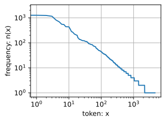
Past the first few words, the curve is close to a straight line on log-log axes. This is Zipf’s law: the frequency \(n_i\) of the \(i\)-th most frequent word obeys
\[n_i \propto \frac{1}{i^\alpha}, \tag{8.3.6}\]
equivalently \(\log n_i = -\alpha \log i + c\) for an exponent \(\alpha\) and constant \(c\). A power law has a heavy tail: a large fraction of all occurrences belongs to words that are individually rare. Does the same hold for word pairs and triples? We can lay all three curves on common axes.
bigrams = ['--'.join(pair) for pair in zip(words[:-1], words[1:])]
trigrams = ['--'.join(tri) for tri in zip(
    words[:-2], words[1:-1], words[2:])]
bigram_freqs = [freq for token, freq in d2l.Vocab(bigrams).token_freqs]
trigram_freqs = [freq for token, freq in d2l.Vocab(trigrams).token_freqs]
d2l.plot([freqs, bigram_freqs, trigram_freqs], xlabel='token: x',
         ylabel='frequency: n(x)', xscale='log', yscale='log',
         legend=['unigram', 'bigram', 'trigram'])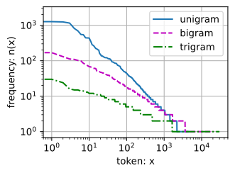
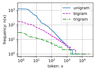
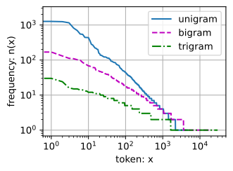
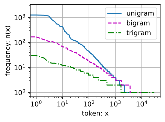
Three observations. First, bigrams and trigrams follow Zipf’s law too, with smaller exponents, so language is power-law distributed at every order of context. Second, the total number of distinct \(n\)-grams is far smaller than \(|\mathcal{V}|^n\): there is a great deal of structure in language, which is why modeling it is possible at all. Third, and decisive for \(n\)-gram models: the curves shift toward count one as \(n\) grows. Most distinct trigrams occur exactly once, so their conditional probability estimates rest on a single observation, and the trigrams of unseen text mostly fall off the table entirely, as we measured above. The tail is where count-based models die. Any approach that estimates each sequence’s probability separately needs exponentially more data as the context grows; models that generalize across related contexts are the way forward.
8.3.4 Perplexity and Bits per Byte
8.3.4.1 Perplexity
Sampling gave us a qualitative readout of model quality; now we need a number. How to obtain one is less obvious than it seems. One way to think about it is to check how surprising the text is to the model. A good language model predicts, with high accuracy, the tokens that come next. Consider the following continuations of the phrase “It is raining”, as proposed by three different language models:
- “It is raining outside”
- “It is raining banana tree”
- “It is raining piouw;kcj pwepoiut”
Example 1 is clearly the best. The words are sensible and logically coherent. While it might not quite accurately reflect which word follows semantically (“in San Francisco” and “in winter” would have been perfectly reasonable extensions), the model captures which kind of word follows. Example 2 is considerably worse, producing a nonsensical extension. Nonetheless, at least the model has learned how to spell words and some degree of correlation between them. Finally, example 3 indicates a poorly trained model that does not fit the data properly.
We might measure the quality of the model by computing the likelihood of a sequence. Unfortunately this is a number that is hard to understand and difficult to compare: shorter sequences are much more likely than longer ones, so evaluating the model on Tolstoy’s magnum opus War and Peace will inevitably produce a much smaller likelihood than on Saint-Exupery’s novella The Little Prince. What is missing is the equivalent of an average.
Information theory supplies it. We defined entropy, surprisal, and cross-entropy when we introduced softmax regression (Section 3.1.3.2.1). If we want to compress text, we can ask about predicting the next token given the current set of tokens: a better language model lets us spend fewer bits per token. So we measure a model by the cross-entropy loss averaged over all \(T\) tokens of a sequence,
\[\frac{1}{T} \sum_{t=1}^T -\log P(x_t \mid x_{t-1}, \ldots, x_1), \tag{8.3.7}\]
where \(P\) is given by the language model and \(x_t\) is the actual token observed at time step \(t\). This makes performance on documents of different lengths comparable. For historical reasons, natural language processing prefers the exponential of Equation 8.3.7, called perplexity (Jelinek et al. 1977):
\[\exp\left(-\frac{1}{T} \sum_{t=1}^T \log P(x_t \mid x_{t-1}, \ldots, x_1)\right).\]
Perplexity is best understood as the geometric mean of the number of real choices the model faces when deciding which token comes next, its effective branching factor. Three reference points make the scale concrete:
- In the best case, the model always assigns the target token probability 1, and the perplexity is 1.
- In the worst case, the model assigns some target token probability 0, and the perplexity is infinite.
- At the baseline, the model predicts a uniform distribution over the vocabulary, and the perplexity equals \(|\mathcal{V}|\), the number of distinct tokens. Storing the sequence without any compression costs exactly this many choices per token, so this is an upper bound that any useful model must beat.
The worst case is not hypothetical: it is what an unsmoothed \(n\)-gram model does on every unseen \(n\)-gram, of which the held-out text is full. Smoothing Equation 8.3.5 exists precisely so that perplexity stays finite. Let’s evaluate our three word-level models on the held-out split.
def eval_nll(model, tokens):
    """Total negative log-likelihood of tokens, in nats."""
    return -sum(math.log(model.prob(tokens[:t], tokens[t]))
                for t in range(len(tokens)))

for n, model in models.items():
    ppl = math.exp(eval_nll(model, words_val) / len(words_val))
    print(f'{n}-gram held-out perplexity: {ppl:8.1f}')
1-gram held-out perplexity: 840.7
2-gram held-out perplexity: 775.1
3-gram held-out perplexity: 2618.1The result should give you pause: the trigram model, which wrote by far the most convincing text, has by far the worst held-out perplexity, and at the shared smoothing constant even the bigram barely improves on the unigram. Both observations result from count sparsity in disguise. When 87% of held-out trigrams are unseen, the trigram model spends most of its time on smoothed near-uniform guesses, and no choice of \(\alpha\) rescues it (the exercises ask you to try). Good-looking samples and good generalization are different things, and the gap between them is memorization. The actual job of a language model is to close that gap, achieving low perplexity on unseen text, and perplexity will be our chief metric for the neural models of the coming sections.
8.3.4.2 Bits per Byte
One subtlety hides in “per token”: perplexity depends on what a token is. A character model chooses among 27 symbols per step while our word model chooses among thousands, so their perplexities are not remotely comparable. Since Section 8.2 taught us that tokenization itself is a design choice, a fair metric must not depend on it. The fix is to change the denominator: divide the total surprisal not by the number of tokens, a tokenizer-dependent quantity, but by the number of bytes of text, a property of the data alone. Measuring surprisal in bits (base-2 logarithms) gives bits per byte,
\[\textrm{bpb} = \frac{1}{B} \sum_{t=1}^T -\log_2 P(x_t \mid x_{t-1}, \ldots, x_1), \tag{8.3.8}\]
where \(B\) is the length of the evaluated text in UTF-8 bytes. This is a compression rate: a model with bits per byte \(b\) can, paired with an arithmetic coder, compress the text to a fraction \(b/8\) of its raw size. One experiment makes the contrast between the two metrics visible: the same model class (a trigram with the same smoothing) estimated on the same training text under three tokenizations, characters, our vocabulary-1,024 BPE from Section 8.2, and words.
bpe = d2l.BPETokenizer(vocab_size=1024, pattern=d2l.BPETokenizer.GPT2_PATTERN)
bpe.train(text[:split])
streams = {'character': (list(text[:split]), list(text[split:]),
                         len(set(text))),
           'BPE (1,024)': (bpe.encode(text[:split]), bpe.encode(text[split:]),
                           bpe.vocab_size),
           'word': (words_train, words_val, vocab_size)}
n_bytes = len(text[split:].encode('utf-8'))
print(f'{"tokenization":>12} {"|V|":>5} {"tokens":>7} {"ppl":>8} {"bpb":>5}')
for name, (train, val, m) in streams.items():
    nll = eval_nll(NGramLM(train, 3, m), val)
    print(f'{name:>12} {m:>5} {len(val):>7} '
          f'{math.exp(nll / len(val)):>8.1f} {nll / math.log(2) / n_bytes:>5.2f}')
tokenization |V| tokens ppl bpb
character 27 17345 6.4 2.68
BPE (1,024) 1024 5509 281.6 2.58
word 4579 3373 2618.1 2.21Judged by perplexity the three models look incomparably different, spanning more than two orders of magnitude; judged by bits per byte they are nearly tied, and the ordering even reverses: the character model has the lowest perplexity yet compresses worst, because at a fixed order \(n\) coarser tokens condition on more actual text. Two words of context reach some fifteen characters back, two characters of context barely finish a syllable. The word model “wins” here only because we quietly told it the held-out vocabulary in advance; the byte-level BPE model needs no such favor, which is one more reason modern models use subword tokenization.
Because bits per byte is tokenizer-independent, it is how modern language modeling runs are compared: a training run with a 50,000-token vocabulary and one with a 200,000-token vocabulary cannot be compared by perplexity at all, but their bits per byte are directly commensurable. The magnitudes are worth remembering. Shannon estimated, using human predictions, that printed English carries around one bit per character (Shannon 1951); strong neural language models now compress diverse web text below one bit per byte, while our best count-based model sits above two. The distance between those numbers is the distance this part of the book travels.
8.3.5 Partitioning Sequences
We close by preparing the data pipeline for the neural language models of the coming sections: they will be trained on the BPE token ids of Section 8.2, consumed as minibatches of fixed-length subsequences.
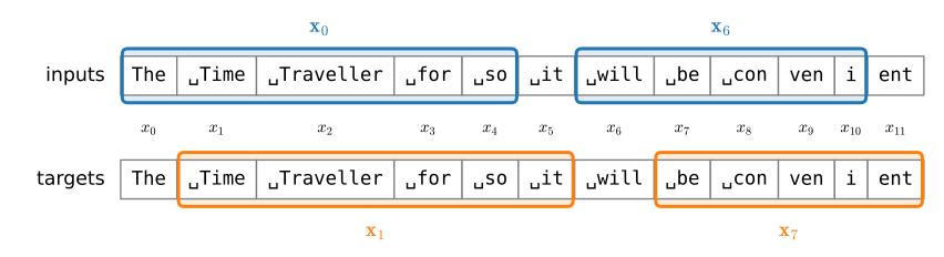
Suppose the corpus is a stream of \(T\) token ids. We form all overlapping subsequences of length \(n\) (here \(n\) plays the role of a sequence length, num_steps, not an \(n\)-gram order): denote by \(\mathbf x_t = [x_t, \ldots, x_{t+n-1}]\) the subsequence starting at position \(t\), giving candidates \(\mathbf x_0, \mathbf x_1, \ldots,
\mathbf x_{T-n-1}\). Since a language model predicts the next token from the tokens so far, the target for input \(\mathbf x_t\) is the same window shifted forward by one position, \(\mathbf x_{t+1}\): while the model reads \(x_t,
\ldots, x_{t+n-1}\) it is trained to emit \(x_{t+1}, \ldots, x_{t+n}\), token by token. Figure 8.3.1 shows two such (input, target) pairs over the actual opening tokens of our corpus. At training time we draw minibatches of pairs at random from the full overlapping collection, which provides the stochasticity that stochastic gradient descent expects without discarding any position in the corpus.
The constructor below assembles the full pipeline: download the corpus, train the tokenizer of Section 8.2 on it (byte-level BPE with the GPT-2 pre-tokenization pattern), encode the corpus into token ids, and lay out all overlapping input and target windows as rows of two aligned arrays. The trained tokenizer remains available as data.tokenizer, so ids can be decoded back into text; data.vocab refers to it as well, so len(data.vocab) gives the vocabulary size in either mode. Passing tokenization='char' selects the character-level pipeline of Section 8.2 instead, which later chapters use for character-level models.
@d2l.add_to_class(d2l.TimeMachine)
def __init__(self, batch_size, num_steps, num_train=10000, num_val=5000,
             tokenization='bpe', vocab_size=1024):
    super(d2l.TimeMachine, self).__init__()
    self.save_hyperparameters()
    raw_text = self._download()
    if tokenization == 'bpe':
        self.tokenizer = d2l.BPETokenizer(
            vocab_size, pattern=d2l.BPETokenizer.GPT2_PATTERN)
        self.tokenizer.train(raw_text)
        corpus, self.vocab = self.tokenizer.encode(raw_text), self.tokenizer
    else:  # 'char': the character-level pipeline
        corpus, self.vocab = self.build(raw_text)
    array = d2l.tensor([corpus[i:i+num_steps+1]
                        for i in range(len(corpus)-num_steps)])
    self.X, self.Y = array[:,:-1], array[:,1:]
Training and validation use disjoint ranges of window positions. The data loader samples minibatches of (input, target) rows at random for training and sequentially for validation.
@d2l.add_to_class(d2l.TimeMachine)
def get_dataloader(self, train):
    idx = slice(0, self.num_train) if train else slice(
        self.num_train, self.num_train + self.num_val)
    return self.get_tensorloader([self.X, self.Y], train, idx)
Each minibatch is a pair of integer arrays of shape (batch_size, num_steps), and the target array is the input array shifted by one token. Decoding a row confirms that the ids really are Wells’ prose, and that input and target are the same text one token apart.
data = d2l.TimeMachine(batch_size=2, num_steps=10)
for X, Y in data.train_dataloader():
    print('X:', X, '\nY:', Y)
    break
print('X[0]:', repr(data.tokenizer.decode([int(i) for i in X[0]])))
print('Y[0]:', repr(data.tokenizer.decode([int(i) for i in Y[0]])))X: tensor([[ 39, 454, 545, 269, 491, 44, 492, 73, 102, 316],
[271, 338, 362, 311, 272, 625, 304, 284, 942, 10]])
Y: tensor([[ 454, 545, 269, 491, 44, 492, 73, 102, 316, 1015],
[ 338, 362, 311, 272, 625, 304, 284, 942, 10, 100]])
X[0]: "'But,' I said, 'If it"
Y[0]: "But,' I said, 'If it travell"X: tf.Tensor(
[[109 754 275 285 298 104 277 286 682 44]
[273 708 650 430 565 776 622 285 256 736]], shape=(2, 10), dtype=int32)
Y: tf.Tensor(
[[754 275 285 298 104 277 286 682 44 277]
[708 650 430 565 776 622 285 256 736 316]], shape=(2, 10), dtype=int32)
X[0]: 'm going to wash and dress,'
Y[0]: ' going to wash and dress, and'X: [[337 321 33 39 280 720 516 360 844 44]
[114 300 270 277 10 99 521 357 270 708]]
Y: [[321 33 39 280 720 516 360 844 44 648]
[300 270 277 10 99 521 357 270 708 349]]
X[0]: "iment!' cried Filby,"
Y[0]: "ent!' cried Filby, who"X: [[ 10. 39. 83. 116. 558. 314. 286. 428. 110. 270.]
[ 10. 10. 39. 89. 276. 324. 294. 285. 965. 313.]]
Y: [[ 39. 83. 116. 558. 314. 286. 428. 110. 270. 33.]
[ 10. 39. 89. 276. 324. 294. 285. 965. 313. 313.]]
X[0]: "\n'Story be damned"
Y[0]: "'Story be damned!"8.3.6 Summary and Discussion
Language models assign probabilities to token sequences, and the chain rule reduces them to next-token prediction, which makes one model a generator, a scorer of hypotheses, and, at scale, an interface to any task expressible as a continuation. \(n\)-gram models implement the conditional with counts under a Markov assumption; they are trivial to estimate and already write locally convincing text, but Zipf’s law guarantees that the count tables go sparse exponentially fast in \(n\), so they memorize rather than generalize, and smoothing can only paper over the zeros. Perplexity, the exponentiated average cross-entropy, is the standard quality metric, interpretable as an effective branching factor; because it is defined per token it cannot compare models with different tokenizers, for which bits per byte is the tokenizer-independent standard. Finally, we prepared the training pipeline used in the rest of this chapter: the corpus becomes one stream of BPE token ids, cut into all overlapping fixed-length windows, with targets shifted by one token and minibatches drawn at random.
Language models scale with data, model size, and compute. Trained on internet-scale corpora, the same next-token objective yields systems that perform tasks from translation to coding when prompted with an appropriate context. We will return to what emerges from that scaling in Section 11.4.1; the next sections build the first neural architectures of that lineage.
8.3.7 Exercises
- [code] Temperature sampling.
NGramLM.sampledraws each next token in proportion to its raw count \(N\). Add a temperature \(\tau > 0\) by drawing in proportion to \(N^{1/\tau}\) instead.- Generate trigram text from the prefix
['the', 'time']at \(\tau \in \{0.3, 1, 3\}\) and describe what changes. - Which distribution over successors does the sampler approach as \(\tau \to 0\), and which as \(\tau \to \infty\)? For a context that occurred exactly once in training, what does the temperature change?
- Generate trigram text from the prefix
- [code] Normalization across lengths. ●
NGramLMhas no end-of-sequence token. Train a bigramNGramLMwith \(\alpha = 1\) andvocab_size=3on a short string over a three-symbol vocabulary. Useproband the chain rule Equation 8.3.2 to sum the probabilities of all sequences of length 2, and separately those of all sequences of length 3.- What does each sum equal, and what do the two sums say about the model as a distribution over sequences whose length is not fixed in advance?
- Add an end-of-sequence token to the vocabulary, so that
vocab_size=4, and append it to the training string. Treat a sequence as complete once it emits this token. Show that the probabilities of all complete sequences now sum to exactly one. Which property of the model rules out probability mass on sequences that never end?
- Dense versus sparse storage. Consider a 5-gram model over a vocabulary of \(|\mathcal{V}| = 50{,}000\) word tokens.
- How many entries does a dense table of the conditional probabilities Equation 8.3.4 contain?
- Suppose instead that only the 5-grams observed in a trillion-token corpus are stored, at 16 bytes per entry. How much memory is needed at most, and what fraction of all possible 5-grams is covered?
- The code in Section 8.3.2 prints the number of distinct word trigrams in the training text and the fraction of held-out trigrams that never occurred in training. The word vocabulary there has \(|\mathcal{V}| = 4{,}579\) types. Compare the fraction of all possible trigrams that occur in training with the fraction of held-out trigrams that do. What does the gap say about the coverage of (b) as an estimate of how often a query on new text finds its 5-gram in the table?
- [code] Smoothing constant. Sweep \(\alpha\) in Equation 8.3.5 over the 19 values \(\alpha = 10^{k/4}\) for \(k = -16, -15, \ldots, 2\), for the unigram, bigram, and trigram word models, and plot held-out perplexity against \(\alpha\) on a logarithmic axis.
- How does the best \(\alpha\) change with \(n\), and why?
- Rank the three models, each at its own best \(\alpha\), by held-out perplexity. How does this ranking differ from the one printed in Section 8.3.4 with the default \(\alpha = 0.01\) of
NGramLM?
- [code] Seen and unseen trigrams. ● Split the held-out positions from the third word on by whether the word trigram ending at that position occurred in training. Take the bigram and the trigram word models, each at its best \(\alpha\) from the sweep of the previous problem, and compute the average negative log-likelihood of each model on each group. On which group is the trigram the better model, and what does this suggest about combining models of different orders?
- Perplexity under skew. A training corpus over ten symbols consists of one symbol 91% of the time and each of the other nine 1% of the time.
- Compute the perplexity of the unigram model estimated from this corpus on a long test text drawn from the same distribution. How does it compare with the vocabulary size of ten?
- The word-level unigram model of Section 8.3.4 chooses among thousands of word types. Read off its held-out perplexity as an effective number of equally likely choices, and explain with Zipf’s law Equation 8.3.6 why this number is far below \(|\mathcal{V}|\).
- Bits per byte from perplexity. A model achieves per-token perplexity \(\textrm{ppl}\) on a text that its tokenizer splits into \(T\) tokens and whose size is \(B\) UTF-8 bytes.
- Show that its bits per byte Equation 8.3.8 equals \[\textrm{bpb} = \frac{T}{B} \log_2 \textrm{ppl}.\]
- Use the formula and the table printed in Section 8.3.4.2 to compute the average number of bytes per token, \(B/T\), for each tokenization. Explain how bits per byte that nearly agree can coexist with perplexities that differ by more than two orders of magnitude.
- What held-out perplexity would the BPE-level trigram need in order to reach one bit per byte?
- Overlapping windows.
d2l.TimeMachinebuilds one row ofnum_steps + 1consecutive tokens for every possible start position in the corpus. The firstnum_stepstokens of a row form a row ofX, and the lastnum_stepstokens form the matching row ofY. The firstnum_trainrows go to training and the nextnum_valrows to validation (Section 8.3.5). Takenum_steps=32,num_train=10000, andnum_val=5000.- Counting input and target tokens together, how many corpus positions do the training rows touch, and how many do the validation rows touch? How many positions do both touch?
- How many times per epoch does a token in the interior of the training range serve as a target?
- How many windows does a partition of the entire corpus of about 66,000 tokens into non-overlapping 32-token windows yield? Compare this partition with the 10,000 overlapping training rows in the number of windows and in the number of distinct corpus positions covered.