%matplotlib inline
from d2l import torch as d2l
import numpy as np
import torch9.2 Gradient Descent
Deep learning usually uses stochastic variants of gradient descent, but the deterministic method exposes the same effects of step size and curvature. A learning rate that causes divergence on a one-dimensional quadratic can cause divergence in a large network for the same reason. Likewise, preconditioning for differently scaled coordinates reappears in the adaptive methods of Section 9.6. This section studies descent direction and step size; Section 9.3 adds gradient noise.
9.2.1 One-Dimensional Gradient Descent
Why should stepping against the gradient reduce the objective at all? The one-dimensional case already contains the answer. Consider a continuously differentiable function \(f: \mathbb{R} \rightarrow \mathbb{R}\). Its Taylor expansion reads
\[f(x + \epsilon) = f(x) + \epsilon f'(x) + \mathcal{O}(\epsilon^2). \tag{9.2.1}\]
For small \(\epsilon\) the function is well approximated by its tangent line, so moving against the derivative should decrease \(f\). Pick a fixed step size \(\eta > 0\), choose \(\epsilon = -\eta f'(x)\), and substitute:
\[f(x - \eta f'(x)) = f(x) - \eta f'^2(x) + \mathcal{O}(\eta^2 f'^2(x)). \tag{9.2.2}\]
Unless the derivative vanishes, the first-order term \(\eta f'^2(x) > 0\) pulls the value down, and we can always choose \(\eta\) small enough for the higher-order remainder to stay negligible. Hence
\[f(x - \eta f'(x)) \lessapprox f(x),\]
and iterating
\[x \leftarrow x - \eta f'(x) \tag{9.2.3}\]
decreases the objective locally when the Taylor remainder is dominated by the first-order term. A global step-size guarantee needs an additional smoothness condition. If \(f'\) is \(L\)-Lipschitz, for example, gradient descent decreases \(f\) for \(0<\eta<2/L\); Chapter 26 proves this result.
To watch the iteration at work we use \(f(x)=x^2\). We know that \(x=0\) is the minimizer, which makes it easy to judge how the iterates behave.
%matplotlib inline
from d2l import jax as d2l
import jax
from jax import numpy as jnp
import numpy as np
def f(x): # Objective function
return x ** 2
def f_grad(x): # Gradient (derivative) of the objective function
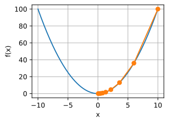
return 2 * xStarting from \(x=10\) with \(\eta=0.2\), ten iterations bring \(x\) close to the optimum.
def gd(eta, f_grad):
    x = 10.0
    results = [x]
    for i in range(10):
        x -= eta * f_grad(x)
        results.append(float(x))
    print(f'epoch 10, x: {x:f}')
    return results

results = gd(0.2, f_grad)
epoch 10, x: 0.060466The progress of optimizing over \(x\) can be plotted as follows.
def show_trace(results, f):
    n = max(abs(min(results)), abs(max(results)))
    f_line = d2l.arange(-n, n, 0.01)
    d2l.set_figsize()
    d2l.plot([f_line, results], [[f(x) for x in f_line], [
        f(x) for x in results]], 'x', 'f(x)', fmts=['-', '-o'])

show_trace(results, f)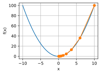
9.2.1.1 Learning Rate
The learning rate \(\eta\) is ours to choose, and both directions of error cost us. Set it too small and \(x\) barely moves: with \(\eta = 0.05\), ten steps leave us far from the solution, and reaching it would take many more.
show_trace(gd(0.05, f_grad), f)epoch 10, x: 3.486784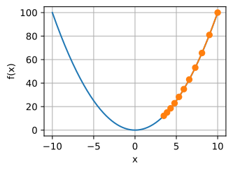
epoch 10, x: 3.486784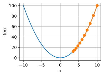
Set it too large and the step \(\left|\eta f'(x)\right|\) outruns the first-order approximation: the remainder \(\mathcal{O}(\eta^2 f'^2(x))\) in Equation 9.2.2 takes over and each update can increase the objective. With \(\eta=1.1\) the iterates overshoot the minimum on every step and gradually diverge.
show_trace(gd(1.1, f_grad), f)epoch 10, x: 61.917364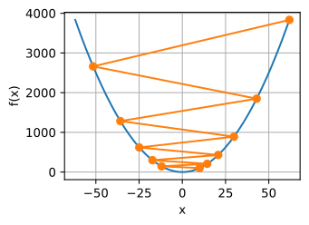
epoch 10, x: 61.917364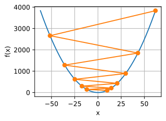
9.2.1.2 Local Minima
On a convex parabola the only risk was the step size. Nonconvex functions add another. Consider \(f(x) = x \cdot \cos(cx)\), which has infinitely many local minima. Depending on the learning rate and on how well conditioned the problem is, gradient descent settles into one of many solutions — and an (unrealistically) large learning rate can bounce the iterate into a poor one.
c = d2l.tensor(0.15 * np.pi)

def f(x):  # Objective function
    return x * d2l.cos(c * x)

def f_grad(x):  # Gradient of the objective function
    return d2l.cos(c * x) - c * x * d2l.sin(c * x)

show_trace(gd(2, f_grad), f)epoch 10, x: -1.528166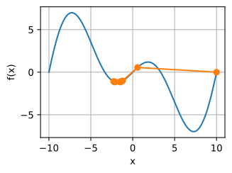
epoch 10, x: -1.528165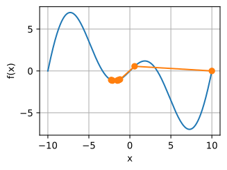
9.2.2 Multivariate Gradient Descent
The same update extends to the multivariate case, \(\mathbf{x} = [x_1, x_2, \ldots, x_d]^\top\), where the objective \(f: \mathbb{R}^d \to \mathbb{R}\) maps vectors to scalars. Its gradient is the vector of \(d\) partial derivatives:
\[\nabla f(\mathbf{x}) = \bigg[\frac{\partial f(\mathbf{x})}{\partial x_1}, \frac{\partial f(\mathbf{x})}{\partial x_2}, \ldots, \frac{\partial f(\mathbf{x})}{\partial x_d}\bigg]^\top. \tag{9.2.4}\]
Each entry \(\partial f(\mathbf{x})/\partial x_i\) measures the rate of change of \(f\) with respect to input \(x_i\). The multivariate Taylor expansion mirrors the one-dimensional one:
\[f(\mathbf{x} + \boldsymbol{\epsilon}) = f(\mathbf{x}) + \mathbf{\boldsymbol{\epsilon}}^\top \nabla f(\mathbf{x}) + \mathcal{O}(\|\boldsymbol{\epsilon}\|^2). \tag{9.2.5}\]
Up to second-order terms, the direction of steepest descent is the negative gradient \(-\nabla f(\mathbf{x})\), and with a suitable learning rate \(\eta > 0\) we obtain the prototypical gradient descent algorithm:
\[\mathbf{x} \leftarrow \mathbf{x} - \eta \nabla f(\mathbf{x}).\]
To see the algorithm in action, take the quadratic \(f(\mathbf{x})=x_1^2+2x_2^2\), a bowl that curves twice as steeply in \(x_2\) as in \(x_1\), whose gradient is \(\nabla f(\mathbf{x}) = [2x_1, 4x_2]^\top\). Starting from the initial position \([-5, -2]\), we track the trajectory of \(\mathbf{x}\). We need two helper functions: the first applies an update rule repeatedly from the fixed starting point, the second draws the trajectory over a contour plot of the objective. Both will be reused throughout this chapter.
def train_2d(trainer, steps=20, f_grad=None):
    """Optimize a 2D objective function with a customized trainer."""
    # `s1` and `s2` are internal state variables used by the stateful
    # optimizers (momentum, Adam) later in this chapter
    x1, x2, s1, s2 = -5, -2, 0, 0
    results = [(x1, x2)]
    for i in range(steps):
        if f_grad:
            x1, x2, s1, s2 = trainer(x1, x2, s1, s2, f_grad)
        else:
            x1, x2, s1, s2 = trainer(x1, x2, s1, s2)
        results.append((x1, x2))
    print(f'epoch {i + 1}, x1: {float(x1):f}, x2: {float(x2):f}')
return resultsdef show_trace_2d(f, results):
"""Show the trace of 2D variables during optimization."""
d2l.set_figsize()
d2l.plt.plot(*zip(*results), '-o', color='#ff7f0e')
x1, x2 = d2l.meshgrid(d2l.arange(-5.5, 1.0, 0.1),
d2l.arange(-3.0, 1.0, 0.1), indexing='ij')
d2l.plt.contour(x1, x2, f(x1, x2), colors='#1f77b4')
d2l.plt.xlabel('x1')
d2l.plt.ylabel('x2')def show_trace_2d(f, results):
"""Show the trace of 2D variables during optimization."""
d2l.set_figsize()
d2l.plt.plot(*zip(*results), '-o', color='#ff7f0e')
x1, x2 = d2l.meshgrid(d2l.arange(-5.5, 1.0, 0.1),
d2l.arange(-3.0, 1.0, 0.1))
d2l.plt.contour(x1, x2, f(x1, x2), colors='#1f77b4')
d2l.plt.xlabel('x1')
d2l.plt.ylabel('x2')With learning rate \(\eta = 0.1\), twenty steps bring \(\mathbf{x}\) near its minimum at \([0, 0]\). Progress is stable but slow. The path bends because the two coordinates contract fastest at different step sizes, a first glimpse of the conditioning problem that Section 9.5 takes up in earnest.
def f_2d(x1, x2):  # Objective function
    return x1 ** 2 + 2 * x2 ** 2

def f_2d_grad(x1, x2):  # Gradient of the objective function
    return (2 * x1, 4 * x2)

def gd_2d(x1, x2, s1, s2, f_grad):
    g1, g2 = f_grad(x1, x2)
    return (x1 - eta * g1, x2 - eta * g2, 0, 0)

eta = 0.1
show_trace_2d(f_2d, train_2d(gd_2d, f_grad=f_2d_grad))epoch 20, x1: -0.057646, x2: -0.000073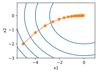
epoch 20, x1: -0.057646, x2: -0.000073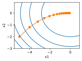
9.2.3 Newton’s Method
The learning-rate experiments in Section 9.2.1.1 showed that one step size may be too small or too large, and the multivariate example showed that the best rate can differ by coordinate. Second-order methods use the objective’s curvature to choose a scaled step. They cannot be applied to deep networks directly, for reasons of cost we quantify below, but they define the ideal that the practical algorithms later in this chapter approximate.
There was no need to stop the Taylor expansion of \(f: \mathbb{R}^d \rightarrow \mathbb{R}\) after the first term. We can write it as
\[f(\mathbf{x} + \boldsymbol{\epsilon}) = f(\mathbf{x}) + \boldsymbol{\epsilon}^\top \nabla f(\mathbf{x}) + \frac{1}{2} \boldsymbol{\epsilon}^\top \nabla^2 f(\mathbf{x}) \boldsymbol{\epsilon} + \mathcal{O}(\|\boldsymbol{\epsilon}\|^3). \tag{9.2.6}\]
Define \(\mathbf{H} \stackrel{\textrm{def}}{=} \nabla^2 f(\mathbf{x})\), the Hessian of \(f\), a \(d \times d\) matrix. For small \(d\) and simple problems \(\mathbf{H}\) is easy to compute; for a deep network it is prohibitively large, with \(\mathcal{O}(d^2)\) entries. For the moment, assume that the Hessian is available and derive the corresponding update.
The minimum of \(f\) satisfies \(\nabla f = 0\). Taking derivatives of Equation 9.2.6 with regard to \(\boldsymbol{\epsilon}\) (following the calculus rules of Section 1.4.2) and ignoring higher-order terms we arrive at
\[\nabla f(\mathbf{x}) + \mathbf{H} \boldsymbol{\epsilon} = 0 \textrm{ and hence } \boldsymbol{\epsilon} = -\mathbf{H}^{-1} \nabla f(\mathbf{x}).\]
Newton’s method is gradient descent with the gradient premultiplied by the inverse Hessian, so the objective’s local curvature determines the scale of each coordinate. As a simple example, for \(f(x) = \frac{1}{2} x^2\) we have \(\nabla f(x) = x\) and \(\mathbf{H} = 1\), so for any \(x\) the update is \(\epsilon = -x\): a single step converges perfectly, with no learning rate to tune. We got a bit lucky here: the Taylor expansion of this \(f\) was exact.
The next experiments consider other objectives. Given a convex hyperbolic cosine function \(f(x) = \cosh(cx)\) for some constant \(c\), the global minimum at \(x=0\) is reached after a few iterations.
c = d2l.tensor(0.5)

def f(x):  # Objective function
    return d2l.cosh(c * x)

def f_grad(x):  # Gradient of the objective function
    return c * d2l.sinh(c * x)

def f_hess(x):  # Hessian of the objective function
    return c**2 * d2l.cosh(c * x)

def newton(eta=1):
    x = 10.0
    results = [x]
    for i in range(10):
        x -= eta * f_grad(x) / f_hess(x)
        results.append(float(x))
    print(f'epoch 10, x: {float(x):f}')
    return results

show_trace(newton(), f)epoch 10, x: 0.000000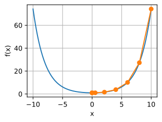
epoch 10, x: 0.000000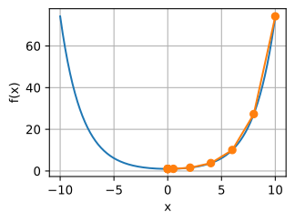
Consider a nonconvex function such as \(f(x) = x \cos(c x)\). Newton’s method divides by the Hessian, so wherever the second derivative is negative, the update moves toward increasing values of \(f\) and may converge to a maximum. The following experiment demonstrates this failure of the undamped Newton update.
c = d2l.tensor(0.15 * np.pi)

def f(x):  # Objective function
    return x * d2l.cos(c * x)

def f_grad(x):  # Gradient of the objective function
    return d2l.cos(c * x) - c * x * d2l.sin(c * x)

def f_hess(x):  # Hessian of the objective function
    return - 2 * c * d2l.sin(c * x) - x * c**2 * d2l.cos(c * x)

show_trace(newton(), f)epoch 10, x: 26.834133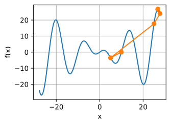
epoch 10, x: 26.834133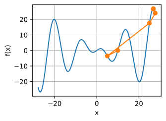
This went spectacularly wrong. How can we fix it? One option is to “repair” the Hessian by taking its absolute value. Another is to bring back the learning rate. This seems to defeat the purpose, but not quite: second-order information still lets us be cautious where curvature is large and take longer steps where the objective is flat. With a slightly smaller learning rate, \(\eta = 0.5\), the damped iteration converges quickly.
show_trace(newton(0.5), f)epoch 10, x: 7.269860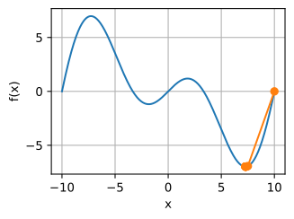
epoch 10, x: 7.269860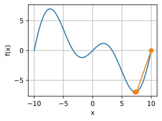
Two facts about Newton’s method are worth carrying away, and both are proved in the appendix rather than here. First, near a minimum with positive curvature it converges quadratically: the number of correct digits roughly doubles at every iteration. Section 26.1.5.3 gives the proof and shows the doubling numerically. Second, nothing rescues the method at deep-learning scale. Storing the Hessian costs \(\mathcal{O}(d^2)\) memory and solving with it \(\mathcal{O}(d^3)\) time, which at \(d \sim 10^9\) parameters means exabytes before the first step. Worse, as the demo above showed in one dimension, a nonconvex objective hands Newton negative curvature that it follows toward saddle points and maxima. The classical remedies are cheaper curvature estimates and safer step rules: quasi-Newton methods such as BFGS rebuild curvature from successive gradient differences (Section 26.1.5.4), line search picks \(\eta\) by trial at run time (Section 26.1.2), and trust regions bound the step instead of the rate (Section 26.1.5.5) (Boyd and Vandenberghe 2004; Nocedal and Wright 2006). None of them fit deep learning as-is; a single line-search trial, for instance, evaluates the objective on the entire dataset.
9.2.3.1 Preconditioning
At large scale, the underlying idea remains useful. Instead of inverting the full Hessian, a preconditioner rescales the update using an inexpensive approximation. The simplest useful choice is the diagonal:
\[\mathbf{x} \leftarrow \mathbf{x} - \eta \, \textrm{diag}(\mathbf{H})^{-1} \nabla f(\mathbf{x}). \tag{9.2.7}\]
This amounts to selecting a separate learning rate for every coordinate. To see why that matters, imagine a model with one parameter measured in millimeters and another in kilometers. Both natural scales are meters, so the two gradients differ by orders of magnitude for no meaningful reason; a single global \(\eta\) must fit both, so it fits neither. Preconditioning removes the mismatch without our ever finding it by hand. This idea drives much of what follows: diagonal preconditioners estimated from gradients rather than second derivatives are the core of AdaGrad and Adam (Section 9.6), and preconditioning whole weight matrices rather than individual coordinates leads to Muon (Section 9.9).
9.2.4 Summary
Gradient descent decreases a differentiable function by stepping against the gradient, and the guarantee holds only while the step is small enough for the first-order Taylor expansion to be trusted. That proviso carries all the trouble: a learning rate chosen too small wastes iterations, one too large overshoots or diverges, and on nonconvex objectives even a well-chosen rate may reach a local rather than global minimum. On a positive-definite quadratic, Newton’s method divides out the curvature and converges in one step, but its \(\mathcal{O}(d^2)\) cost and its attraction to saddle points rule it out for deep networks. The rest of this chapter builds cheap, gradient-estimated stand-ins for that ideal.
9.2.5 Exercises
[code] Learning-rate sweep.
gdruns ten steps from \(x_0 = 10\). Extend it to run at most 100 steps and to stop as soon as \(|x| < 10^{-3}\). Run it on \(f(x) = x^2\) and on \(f(x) = |x|^{1.5}\) at \(\eta \in \{0.01, 0.1, 0.5, 0.9, 1.1\}\).- Tabulate, for each of the ten runs, the number of steps until the stopping test holds, or, for a run that misses the test within 100 steps, whether \(|x|\) grew without bound or stayed bounded.
- For \(f(x) = x^2\), derive the range of learning rates for which the iteration converges from every start and the learning rate that reaches the minimum in one step.
- The second derivative of \(|x|^{1.5}\) is unbounded near the origin. Explain what the iterates do close to \(0\) at any fixed \(\eta\), and why the stopping test is reached late or not at all.
[code] Bisection line search. A convex differentiable \(f\) on \([a, b]\) can be minimized by bisection: evaluate the sign of \(f'\) at the midpoint and keep \([a, (a+b)/2]\) or \([(a+b)/2, b]\) accordingly.
- Explain why the sign of \(f'\) at one point suffices to choose the half, whereas comparing the values \(f(a)\), \(f((a+b)/2)\), and \(f(b)\) does not.
- Derive the number of iterations needed to shrink the interval to a width \(\epsilon\).
- Implement the method and apply it to \(f(x) = \log(\exp(x) + \exp(-2x - 3))\) on \([-5, 5]\) until the interval is narrower than \(10^{-6}\). Modify
gdto start at \(x_0 = 5\) and to stop once \(|f'(x)| < 10^{-6}\), find the fixed learning rate that minimizes its step count on the same function, and compare that count with the bisection count.
[code] Newton’s convergence order. ● In Section 9.2.3,
newtonconverges in a few steps on \(f(x) = \cosh(cx)\). Run it with \(c = 0.5\) from \(x_0 = 10\) and record \(|x_t|\) after every step.- From the last steps before \(x_t\) reaches \(0\) in floating point, estimate the order \(p\) in \(|x_{t+1}| \approx C |x_t|^p\). Where does this fast phase begin, and what governs the steps before it?
- Derive \(p\) and \(C\) from the Taylor expansion of the update \(x - \tanh(cx)/c\) around \(0\), and reconcile \(p\) with the quadratic rate stated in Section 26.1.5.3.
[code] Damped Newton steps. In Section 9.2.3,
newtonheads for a maximum of \(f(x) = x\cos(cx)\) unless damped. On \(x\cos(cx)\) from \(x_0 = 10\), sweep the damping \(\eta \in \{0.25, 0.5, 0.75, 1\}\). Which runs end at a minimum, and what is the sign off_hessalong the paths of those that do not?[code] Stale Hessian factorizations. ● A Newton step in \(d\) dimensions can reuse the Hessian factorization of an earlier step. Minimize \(f(\mathbf{x}) = \sum_{i=1}^{n} \cosh(c\, \mathbf{a}_i^\top \mathbf{x})\) with \(n = 200\), \(d = 50\), \(c = 0.5\), directions \(\mathbf{a}_i\) with independent standard Gaussian entries, and \(\mathbf{x}_0 = \mathbf{1}\). Its minimum is \(f^\star = n\) at \(\mathbf{x} = \mathbf{0}\). Charge \(4nd\) operations per gradient, \(nd^2\) per Hessian evaluation, \(d^3/3\) per Cholesky factorization, and \(2d^2\) per pair of triangular solves. Evaluate and factor the Hessian on every step, every 5 steps, and every 20 steps, reusing the stale factorization in between. Plot \(f(\mathbf{x}_t) - f^\star\) against the cumulative operation count rather than the iteration count. Which variant reaches \(10^{-8}\) first, and which of the four costs dominates its total?
Adapted from Stephen Boyd and Lieven Vandenberghe, Convex Optimization, Exercise 9.31(a).
[code] Diagonal preconditioning. The update Equation 9.2.7 of Section 9.2.3.1 gives every coordinate its own learning rate.
- Design an objective on \(\mathbb{R}^2\) by scaling the two coordinates of a quadratic bowl so that the condition number of its Hessian is at least \(100\). Derive the range of learning rates for which plain gradient descent converges and the learning rate that minimizes the larger of the two per-coordinate contraction factors. Report the number of steps gradient descent needs at that rate to reach \(\|\mathbf{x}\| < 10^{-3}\) from the starting point of
d2l.train_2d. - Implement Equation 9.2.7 as a trainer for
d2l.train_2dand repeat the measurement at \(\eta = 1\) and at \(\eta = 0.5\). Explain why the step count no longer depends on the scaling you chose. - Rotate the coordinates of your quadratic by \(45^\circ\) and rerun plain gradient descent, the preconditioned trainer, and Newton’s method. Which of the three are unaffected by the rotation? Explain the behavior of the diagonal preconditioner from the entries of the rotated Hessian.
- Design an objective on \(\mathbb{R}^2\) by scaling the two coordinates of a quadratic bowl so that the condition number of its Hessian is at least \(100\). Derive the range of learning rates for which plain gradient descent converges and the learning rate that minimizes the larger of the two per-coordinate contraction factors. Report the number of steps gradient descent needs at that rate to reach \(\|\mathbf{x}\| < 10^{-3}\) from the starting point of
[code] Absolute-curvature preconditioning. Replace \(\textrm{diag}(\mathbf{H})^{-1}\) in Equation 9.2.7 by \(|\textrm{diag}(\mathbf{H})|^{-1}\) and run this variant at \(\eta = 1\) on the nonconvex \(f(x_1, x_2) = x_1 \cos(c x_1) + x_2 \cos(c x_2)\) with \(c = 0.15\pi\) from the starting point of
d2l.train_2d. Show that every update direction is a descent direction. Does every step decrease \(f\)? Explain the size of the largest step of the run.[code] Counting local minima. The objective \(f(x) = x\cos(cx)\) with \(c = 0.15\pi\) of Section 9.2.1.2 has many local minima, each with its own basin of attraction.
- Locate every local minimum of \(f\) in the open interval \((-20, 20)\) and its value. How does the number of local minima grow as the interval widens?
- Let
gdtake its starting point as an argument. Run 20 steps from \(x_0 \in \{-10, 5, 10\}\) at \(\eta \in \{0.5, 1, 2\}\) and record the minimum each run ends near, if any. Which combinations reach the lowest local minimum in \((-20, 20)\), and why does the largest learning rate change basins?
Certifying the lowest minimum. ● Modify the objective \(f(x) = x\cos(cx)\) with \(c = 0.15\pi\) of Section 9.2.1.2 so that its local minima in \((-20, 20)\) differ in value by at most \(10^{-3}\) except for one. Explain why any method that uses only \(f\) and \(f'\) at the points it visits must then visit every basin before it can certify which local minimum is lowest.