%matplotlib inline
from d2l import torch as d2l
import math
import torch
from torch import nn17.2 Training Energy-Based Models
The partition function of Equation 17.1.1 cannot be computed in high dimension, yet energy-based models are trained by maximum likelihood. This section explains how. The gradient of the log-likelihood does not contain \(Z(\boldsymbol{\theta})\) itself but an expectation under the model, and an expectation can be estimated from samples. Producing those samples is the work of Markov chain Monte Carlo, and running a Markov chain inside every parameter update is the cost that the later sections of this chapter remove. The presentation follows lecture 11 of Kuleshov (2023) .
%matplotlib inline
from d2l import jax as d2l
import math
import jax
import jax.flatten_util
from jax import numpy as jnp
from flax import nnx
import optax
17.2.1 The Running Example
The two-dimensional experiments of this chapter share one target distribution: a mixture of three isotropic Gaussians in the plane with unequal weights. Two properties make it useful. Its density and its score are known in closed form, so every learned quantity can be compared with the truth: a model that provides a likelihood by the log-likelihood it assigns to held-out samples, and a score model by its distance from the true score. Its structure is multimodal with separated modes, which is the situation in which sampling methods have trouble and mode weights become measurable. The class below stores the parameters and evaluates the log-density and its gradient with respect to the input in closed form; both formulas also cover the distribution of a mixture sample after it is scaled and perturbed by Gaussian noise, a case that the score-based sections need. It is saved to the d2l library because the two-dimensional experiments of the later sections use it.
class GaussianMixture:
    """A mixture of isotropic Gaussians with closed-form density and score."""
    def __init__(self, means, weights, std):
        self.means = torch.as_tensor(means, dtype=torch.float32)
        self.weights = torch.as_tensor(weights, dtype=torch.float32)
        self.std = std

    def sample(self, n):
        k = torch.multinomial(self.weights, n, replacement=True)
        return self.means[k] + self.std * torch.randn(n, self.means.shape[1])

    def log_prob(self, x, scale=1.0, sigma=0.0):
        """Log density of scale * x0 + sigma * eps, where x0 is a mixture draw."""
        var = (scale * self.std) ** 2 + sigma ** 2
        d2 = ((x[:, None, :] - scale * self.means[None]) ** 2).sum(-1)
        logs = (torch.log(self.weights)[None] - d2 / (2 * var)
                - 0.5 * x.shape[-1] * math.log(2 * math.pi * var))
        return torch.logsumexp(logs, 1)

    def score(self, x, scale=1.0, sigma=0.0):
        """The gradient of log_prob with respect to x, in closed form."""
        var = (scale * self.std) ** 2 + sigma ** 2
        d2 = ((x[:, None, :] - scale * self.means[None]) ** 2).sum(-1)
        r = torch.softmax(torch.log(self.weights)[None] - d2 / (2 * var), 1)
        return (r[:, :, None]
                * (scale * self.means[None] - x[:, None, :])).sum(1) / var
class GaussianMixture:
"""A mixture of isotropic Gaussians with closed-form density and score."""
def __init__(self, means, weights, std):
self.means = jnp.asarray(means, dtype=jnp.float32)
self.weights = jnp.asarray(weights, dtype=jnp.float32)
self.std = std
def sample(self, key, n):
k1, k2 = jax.random.split(key)
k = jax.random.choice(k1, len(self.weights), (n,), p=self.weights)
return self.means[k] + self.std * jax.random.normal(
k2, (n, self.means.shape[1]))
def log_prob(self, x, scale=1.0, sigma=0.0):
"""Log density of scale * x0 + sigma * eps, where x0 is a mixture draw."""
var = (scale * self.std) ** 2 + sigma ** 2
d2 = ((x[:, None, :] - scale * self.means[None]) ** 2).sum(-1)
logs = (jnp.log(self.weights)[None] - d2 / (2 * var)
- 0.5 * x.shape[-1] * math.log(2 * math.pi * var))
return jax.nn.logsumexp(logs, 1)
def score(self, x, scale=1.0, sigma=0.0):
"""The gradient of log_prob with respect to x, in closed form."""
var = (scale * self.std) ** 2 + sigma ** 2
d2 = ((x[:, None, :] - scale * self.means[None]) ** 2).sum(-1)
r = jax.nn.softmax(jnp.log(self.weights)[None] - d2 / (2 * var), 1)
return (r[:, :, None]
* (scale * self.means[None] - x[:, None, :])).sum(1) / varThe components sit at the corners of a triangle with a common standard deviation of \(0.5\) and weights \(0.5\), \(0.3\), and \(0.2\), so the modes are about five units, ten standard deviations, apart. We draw two thousand training points and two thousand test points. The negative log-likelihood of the test set under the true density, about \(2.5\) nats per point, is the value a perfect model would attain up to sampling error, and every model below is measured against it.
torch.manual_seed(0)
mix = GaussianMixture(means=[[-2.5, -1.5], [2.5, -1.5], [0.0, 2.5]],
                      weights=[0.5, 0.3, 0.2], std=0.5)
data, test = mix.sample(2000), mix.sample(2000)
print(f'test NLL under the true density: {-mix.log_prob(test).mean():.3f} nats')
d2l.set_figsize((3.5, 3.5))
d2l.plt.scatter(data[:, 0], data[:, 1], s=4)
d2l.plt.xlabel('$x_1$'), d2l.plt.ylabel('$x_2$');
test NLL under the true density: 2.506 nats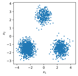
key = jax.random.PRNGKey(0)
mix = GaussianMixture(means=[[-2.5, -1.5], [2.5, -1.5], [0.0, 2.5]],
                      weights=[0.5, 0.3, 0.2], std=0.5)
key, k1, k2 = jax.random.split(key, 3)
data, test = mix.sample(k1, 2000), mix.sample(k2, 2000)
print(f'test NLL under the true density: {-mix.log_prob(test).mean():.3f} nats')
d2l.set_figsize((3.5, 3.5))
d2l.plt.scatter(data[:, 0], data[:, 1], s=4)
d2l.plt.xlabel('$x_1$'), d2l.plt.ylabel('$x_2$');
test NLL under the true density: 2.474 nats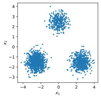
17.2.2 The Maximum-Likelihood Gradient
Consider an energy-based model \(p_{\boldsymbol{\theta}}(\mathbf{x}) = \exp(-E_{\boldsymbol{\theta}}(\mathbf{x})) / Z(\boldsymbol{\theta})\) and a training set \(\mathbf{x}_1, \ldots, \mathbf{x}_n\). The average log-likelihood separates into a term that depends on the data and a term that does not:
\[ \frac{1}{n} \sum_{i=1}^{n} \log p_{\boldsymbol{\theta}}(\mathbf{x}_i) = -\frac{1}{n} \sum_{i=1}^{n} E_{\boldsymbol{\theta}}(\mathbf{x}_i) - \log Z(\boldsymbol{\theta}). \tag{17.2.1}\]
The first term is an average of network outputs and is differentiated by backpropagation. The second term is the logarithm of an intractable integral. Its gradient, however, has a usable form. Differentiating under the integral sign,
\[ \nabla_{\boldsymbol{\theta}} \log Z(\boldsymbol{\theta}) = \frac{1}{Z(\boldsymbol{\theta})} \int \nabla_{\boldsymbol{\theta}} \exp(-E_{\boldsymbol{\theta}}(\mathbf{x}))\, d\mathbf{x} = \int \frac{\exp(-E_{\boldsymbol{\theta}}(\mathbf{x}))}{Z(\boldsymbol{\theta})} \big(-\nabla_{\boldsymbol{\theta}} E_{\boldsymbol{\theta}}(\mathbf{x})\big)\, d\mathbf{x} = -\mathbb{E}_{\mathbf{x} \sim p_{\boldsymbol{\theta}}}\big[\nabla_{\boldsymbol{\theta}} E_{\boldsymbol{\theta}}(\mathbf{x})\big]. \tag{17.2.2}\]
The gradient of the log-partition function is minus the expectation, under the model, of the gradient of the energy. Substituting into Equation 17.2.1 gives the gradient of the average log-likelihood,
\[ \nabla_{\boldsymbol{\theta}} \frac{1}{n} \sum_{i=1}^{n} \log p_{\boldsymbol{\theta}}(\mathbf{x}_i) = -\,\mathbb{E}_{\mathbf{x} \sim p_{\textrm{data}}}\big[\nabla_{\boldsymbol{\theta}} E_{\boldsymbol{\theta}}(\mathbf{x})\big] + \mathbb{E}_{\mathbf{x} \sim p_{\boldsymbol{\theta}}}\big[\nabla_{\boldsymbol{\theta}} E_{\boldsymbol{\theta}}(\mathbf{x})\big], \tag{17.2.3}\]
where the first expectation is over the empirical distribution of the training set. A gradient ascent step therefore moves the parameters to lower the energy at the data and to raise it at samples from the current model. The two contributions are called the positive phase and the negative phase. Training stops moving when the two expectations agree, so the learned model matches the data in the statistics \(\nabla_{\boldsymbol{\theta}} E_{\boldsymbol{\theta}}\). For an exponential family, \(E_{\boldsymbol{\theta}}(\mathbf{x}) = -\boldsymbol{\theta}^\top \mathbf{f}(\mathbf{x})\) with sufficient statistics \(\mathbf{f}\), the gradient reduces to \(\mathbb{E}_{\textrm{data}}[\mathbf{f}(\mathbf{x})] - \mathbb{E}_{\boldsymbol{\theta}}[\mathbf{f}(\mathbf{x})]\), the log-likelihood is concave, and the maximum-likelihood solution matches the moments of the data (Kuleshov 2023). Figure 17.2.1 shows the two phases acting on a one-dimensional energy.
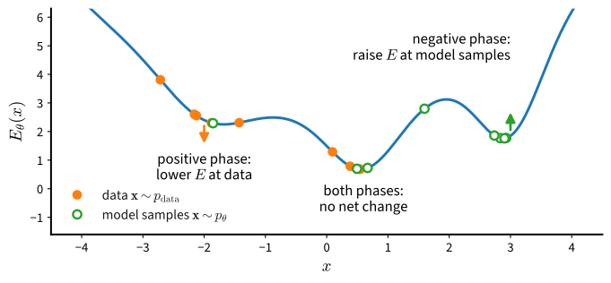
Equation Equation 17.2.3 changes the question. The update does not need the value of \(Z(\boldsymbol{\theta})\); it needs samples from \(p_{\boldsymbol{\theta}}\) to estimate the negative phase. In two dimensions we can check the identity numerically before relying on it, because there the integral can be computed on a grid.
17.2.2.1 A Quadrature Reference in Two Dimensions
The energy below is a small multilayer perceptron with a quadratic term that keeps \(\exp(-E_{\boldsymbol{\theta}})\) integrable. A grid of \(100 \times 100\) points on \([-6, 6]^2\) has spacing \(0.12\), a quarter of the component standard deviation, and quadrature on this grid evaluates \(\log Z(\boldsymbol{\theta})\) accurately enough for every purpose in this section (Exercise 6 of Section 17.1 quantifies the error). Here and below the model is normalized over this square, and the data distribution is taken to be the mixture restricted to it, which changes its density inside the square by about one part in \(10^{12}\). With \(\log Z\) available, the negative log-likelihood Equation 17.2.1 can be minimized directly, for as many updates as the sampling-based training later in the section and with a linearly decaying learning rate. The result is a reference: the fit reached when \(\log Z(\boldsymbol{\theta})\) and its gradient are computed by quadrature. Every sampling-based method below estimates that gradient from model samples instead, and approximates this fit.
class EnergyNet(nn.Module):
    def __init__(self, hidden=64):
        super().__init__()
        self.net = nn.Sequential(nn.Linear(2, hidden), nn.SiLU(),
                                 nn.Linear(hidden, hidden), nn.SiLU(),
                                 nn.Linear(hidden, 1))

    def forward(self, x):  # the quadratic term keeps exp(-E) integrable
        return self.net(x).squeeze(-1) + (x ** 2).sum(-1) / 32

axis = torch.linspace(-6, 6, 100)
grid = torch.stack(torch.meshgrid(axis, axis, indexing='ij'), -1).reshape(-1, 2)
log_cell = 2 * math.log(axis[1] - axis[0])

def log_Z(energy):  # quadrature: possible only because d = 2
    return torch.logsumexp(-energy(grid), 0) + log_cell

def nll(energy, x):
    with torch.no_grad():
        return (energy(x).mean() + log_Z(energy)).item()

torch.manual_seed(1)
energy_mle = EnergyNet()
optimizer = torch.optim.Adam(energy_mle.parameters(), lr=3e-3)
for step in range(3000):
    optimizer.param_groups[0]['lr'] = 3e-3 * (1 - step / 3000)  # linear decay
    x = data[torch.randint(0, len(data), (500,))]
    loss = energy_mle(x).mean() + log_Z(energy_mle)  # negative log-likelihood
    optimizer.zero_grad(), loss.backward(), optimizer.step()
print(f'test NLL with the grid normalizer: {nll(energy_mle, test):.3f} nats')
test NLL with the grid normalizer: 2.511 natsclass EnergyNet(nnx.Module):
def __init__(self, hidden=64, rngs=None):
self.h1 = nnx.Linear(2, hidden, rngs=rngs)
self.h2 = nnx.Linear(hidden, hidden, rngs=rngs)
self.out = nnx.Linear(hidden, 1, rngs=rngs)
def __call__(self, x): # the quadratic term keeps exp(-E) integrable
h = nnx.silu(self.h2(nnx.silu(self.h1(x))))
return self.out(h)[..., 0] + (x ** 2).sum(-1) / 32
axis = jnp.linspace(-6, 6, 100)
grid = jnp.stack(jnp.meshgrid(axis, axis, indexing='ij'), -1).reshape(-1, 2)
log_cell = 2 * math.log(axis[1] - axis[0])
def log_Z(energy): # quadrature: possible only because d = 2
return jax.nn.logsumexp(-energy(grid), 0) + log_cell
@nnx.jit
def nll(energy, x):
return energy(x).mean() + log_Z(energy)
@nnx.jit
def mle_step(energy, optimizer, x):
def loss_fn(model): # negative log-likelihood
return model(x).mean() + log_Z(model)
loss, grads = nnx.value_and_grad(loss_fn)(energy)
optimizer.update(energy, grads)
return loss
energy_mle = EnergyNet(rngs=nnx.Rngs(1))
schedule = optax.linear_schedule(3e-3, 0.0, 3000) # linear decay
optimizer = nnx.Optimizer(energy_mle, optax.adam(schedule), wrt=nnx.Param)
for step in range(3000):
key, subkey = jax.random.split(key)
x = data[jax.random.randint(subkey, (500,), 0, len(data))]
mle_step(energy_mle, optimizer, x)
print(f'test NLL with the grid normalizer: {nll(energy_mle, test):.3f} nats')test NLL with the grid normalizer: 2.480 natsThe test negative log-likelihood lands within a few hundredths of a nat of the true density’s value. The gap is an estimate of the Kullback–Leibler divergence from the restricted data distribution to the model (Section 27.3.2.1), so this energy network can represent the mixture almost exactly when the normalizer is available.
17.2.2.2 Checking the Gradient Identity
Identity Equation 17.2.2 equates two computations that look nothing alike: the gradient of the quadrature estimate of \(\log Z\), obtained by backpropagating through the sum over the grid, and the negative average gradient of the energy at samples from the model. On the grid, the model is a categorical distribution with probabilities proportional to \(\exp(-E_{\boldsymbol{\theta}})\), and this grid model can be sampled exactly. The cell compares the two gradients as the number of samples grows.
def flat_grad(scalar, params):
    return torch.cat([g.reshape(-1) for g in torch.autograd.grad(scalar, params)])

params = list(energy_mle.parameters())
grad_log_Z = flat_grad(log_Z(energy_mle), params)
with torch.no_grad():
    probs = torch.softmax(-energy_mle(grid), 0)  # p_theta on the grid
torch.manual_seed(2)
for n in (100, 1000, 10000):
    x = grid[torch.multinomial(probs, n, replacement=True)]  # x ~ p_theta
    grad_mc = flat_grad(-energy_mle(x).mean(), params)  # -E_p[grad E]
    print(f'{n:>6d} model samples: relative error '
          f'{(grad_mc - grad_log_Z).norm() / grad_log_Z.norm():.3f}')
100 model samples: relative error 0.150
1000 model samples: relative error 0.060
10000 model samples: relative error 0.010def flat_grad(fn, energy):
return jax.flatten_util.ravel_pytree(nnx.grad(fn)(energy))[0]
grad_log_Z = flat_grad(log_Z, energy_mle)
probs = jax.nn.softmax(-energy_mle(grid), 0) # p_theta on the grid
for n in (100, 1000, 10000):
key, subkey = jax.random.split(key)
x = grid[jax.random.choice(subkey, len(grid), (n,), p=probs)] # x ~ p_theta
grad_mc = flat_grad(lambda m: -m(x).mean(), energy_mle) # -E_p[grad E]
print(f'{n:>6d} model samples: relative error '
f'{jnp.linalg.norm(grad_mc - grad_log_Z) / jnp.linalg.norm(grad_log_Z):.3f}') 100 model samples: relative error 0.091
1000 model samples: relative error 0.042
10000 model samples: relative error 0.009The relative error falls roughly as \(1 / \sqrt{n}\), as a Monte Carlo estimate should, and is down to a few percent or less with ten thousand samples. The identity holds; what remains is to produce samples from \(p_{\boldsymbol{\theta}}\) when no grid is available.
17.2.3 Sampling by Markov Chain Monte Carlo
Sampling from a density known only up to a constant is the problem that Markov chain Monte Carlo (MCMC) solves. Section 27.4.3 introduced the method for Bayesian posteriors, which have the same form: a tractable unnormalized density and an intractable normalizer. We recall the definitions needed here and then specialize to energies.
17.2.3.1 Markov Chains and Stationary Distributions
A Markov chain is a sequence of random states \(\mathbf{x}^{(0)}, \mathbf{x}^{(1)}, \ldots\) in which each state is drawn from a transition kernel \(T(\mathbf{x}' \mid \mathbf{x})\) that depends only on the current state. If the state at step \(t\) has distribution \(\pi_t\), the state at step \(t + 1\) has distribution \(\pi_{t+1}(\mathbf{x}') = \int T(\mathbf{x}' \mid \mathbf{x})\, \pi_t(\mathbf{x})\, d\mathbf{x}\). A distribution \(\pi\) is stationary if this map leaves it unchanged. A sufficient condition for stationarity is detailed balance,
\[ \pi(\mathbf{x})\, T(\mathbf{x}' \mid \mathbf{x}) = \pi(\mathbf{x}')\, T(\mathbf{x} \mid \mathbf{x}') \quad \textrm{for all } \mathbf{x}, \mathbf{x}', \tag{17.2.4}\]
which states that under \(\pi\) the flow of probability from \(\mathbf{x}\) to \(\mathbf{x}'\) equals the flow back. Integrating both sides over \(\mathbf{x}\), and using that \(T(\cdot \mid \mathbf{x}')\) integrates to one, gives \(\int \pi(\mathbf{x}) T(\mathbf{x}' \mid \mathbf{x})\, d\mathbf{x} = \pi(\mathbf{x}')\), which is stationarity. The plan of MCMC is to construct a kernel whose stationary distribution is the model \(p_{\boldsymbol{\theta}}\), run the chain long enough that its state distribution has approached the stationary one, and treat subsequent states as model samples. Convergence to the stationary distribution from essentially any starting state holds under two further conditions, that every region can be reached from every other (irreducibility) and that the chain does not cycle with a fixed period (aperiodicity), which the constructions below satisfy for smooth positive densities; MacKay (2003) gives a careful account. The number of steps needed to approach stationarity, the mixing time, is the quantity that decides whether the method is practical.
17.2.3.2 Metropolis–Hastings
The Metropolis–Hastings algorithm (Metropolis et al. 1953; Hastings 1970) builds such a kernel from any proposal distribution \(Q(\mathbf{x}' \mid \mathbf{x})\) that can be sampled and evaluated. From the current state \(\mathbf{x}\), draw a proposal \(\mathbf{x}' \sim Q(\cdot \mid \mathbf{x})\) and accept it with probability
\[ A(\mathbf{x}' \mid \mathbf{x}) = \min\left\{1,\ \frac{p_{\boldsymbol{\theta}}(\mathbf{x}')\, Q(\mathbf{x} \mid \mathbf{x}')}{p_{\boldsymbol{\theta}}(\mathbf{x})\, Q(\mathbf{x}' \mid \mathbf{x})}\right\}; \tag{17.2.5}\]
otherwise the chain stays at \(\mathbf{x}\). The density enters only through the ratio \(p_{\boldsymbol{\theta}}(\mathbf{x}') / p_{\boldsymbol{\theta}}(\mathbf{x}) = \exp(E_{\boldsymbol{\theta}}(\mathbf{x}) - E_{\boldsymbol{\theta}}(\mathbf{x}'))\), so the normalizer cancels. For a symmetric proposal such as a Gaussian random walk \(\mathbf{x}' = \mathbf{x} + \tau \boldsymbol{\xi}\) with \(\boldsymbol{\xi} \sim \mathcal{N}(\mathbf{0}, I)\), the proposal ratio is one and the rule becomes: always accept a move to lower energy, and accept a move to higher energy with probability \(\exp(-\Delta E)\), where \(\Delta E = E_{\boldsymbol{\theta}}(\mathbf{x}') - E_{\boldsymbol{\theta}}(\mathbf{x})\) is the increase in energy.
The kernel satisfies detailed balance with respect to \(p_{\boldsymbol{\theta}}\). For \(\mathbf{x}' \neq \mathbf{x}\) the kernel is \(T(\mathbf{x}' \mid \mathbf{x}) = Q(\mathbf{x}' \mid \mathbf{x}) A(\mathbf{x}' \mid \mathbf{x})\). If the ratio in Equation 17.2.5 is at most one, then \(A(\mathbf{x}' \mid \mathbf{x})\) equals that ratio and \(A(\mathbf{x} \mid \mathbf{x}') = 1\), so
\[ p_{\boldsymbol{\theta}}(\mathbf{x})\, Q(\mathbf{x}' \mid \mathbf{x})\, A(\mathbf{x}' \mid \mathbf{x}) = p_{\boldsymbol{\theta}}(\mathbf{x}')\, Q(\mathbf{x} \mid \mathbf{x}') = p_{\boldsymbol{\theta}}(\mathbf{x}')\, Q(\mathbf{x} \mid \mathbf{x}')\, A(\mathbf{x} \mid \mathbf{x}'), \]
which is Equation 17.2.4; if the ratio exceeds one, the same computation applies with the roles of \(\mathbf{x}\) and \(\mathbf{x}'\) exchanged, and rejected moves contribute equally to both sides because they leave the state unchanged. Gibbs sampling (Geman and Geman 1984) is the special case in which the proposal resamples one coordinate from its exact conditional distribution given the others; its acceptance probability is always one, and it is the standard sampler for the discrete models of Section 17.1, whose conditionals are tractable.
The sampler is a few lines. It runs many chains in parallel, one per row of its input, and returns the final states together with the acceptance rate. An optional argument, box, confines the chains to a square by rejecting every proposal that leaves it. This is the acceptance rule above applied to the model restricted to the square, whose density is zero outside it; the training experiment below uses it.
def metropolis_hastings(energy, x, steps, step_size, box=math.inf):
    """Random-walk Metropolis-Hastings on exp(-energy), one chain per row.
    Proposals outside the square [-box, box]^2 are rejected."""
    accepted = 0.0
    with torch.no_grad():
        e = energy(x)
        for _ in range(steps):
            proposal = x + step_size * torch.randn_like(x)
            e_prop = energy(proposal)
            log_u = torch.log(torch.rand(len(x), device=x.device))
            accept = ((log_u < e - e_prop)  # probability min(1, p'/p)
                      & (proposal.abs() <= box).all(-1))
            x = torch.where(accept[:, None], proposal, x)
            e = torch.where(accept, e_prop, e)
            accepted += accept.float().mean().item()
    return x, accepted / steps
@nnx.jit
def mh_step(energy, x, e, key, step_size, box):
k1, k2 = jax.random.split(key)
proposal = x + step_size * jax.random.normal(k1, x.shape)
e_prop = energy(proposal)
log_u = jnp.log(jax.random.uniform(k2, (len(x),)))
accept = ((log_u < e - e_prop) # probability min(1, p'/p)
& (jnp.abs(proposal) <= box).all(-1))
x = jnp.where(accept[:, None], proposal, x)
e = jnp.where(accept, e_prop, e)
return x, e, accept.mean()
def metropolis_hastings(energy, x, key, steps, step_size, box=math.inf):
"""Random-walk Metropolis-Hastings on exp(-energy), one chain per row.
Proposals outside the square [-box, box]^2 are rejected."""
e, accepted = energy(x), 0.0
for _ in range(steps):
key, subkey = jax.random.split(key)
x, e, rate = mh_step(energy, x, e, subkey, step_size, box)
accepted += float(rate)
return x, accepted / steps17.2.3.3 The Step Size Trades Acceptance against Mixing
Before using the sampler inside training, we run it on a target whose samples we can check: the energy \(-\log p\) of the mixture itself. Two thousand chains start from a broad Gaussian and run for two thousand steps at three proposal scales. We record the acceptance rate, the fraction of chains that end nearest to each component mean, which should match the weights \(0.5\), \(0.3\), \(0.2\), and the mean squared distance from a chain to its nearest mean, which for a two-dimensional Gaussian with standard deviation \(0.5\) should be \(2 \times 0.25 = 0.5\).
def mode_weights(x):
    """The fraction of points closest to each component mean."""
    d2 = ((x[:, None, :] - mix.means[None]) ** 2).sum(-1)
    return [round(w, 3) for w in
            (torch.bincount(d2.argmin(1), minlength=3) / len(x)).tolist()]

true_energy = lambda x: -mix.log_prob(x)
torch.manual_seed(3)
x_init = 3 * torch.randn(2000, 2)
print(f'true mode weights: {[round(w, 3) for w in mix.weights.tolist()]}')
for step_size in (0.25, 1.0, 4.0):
    x, rate = metropolis_hastings(true_energy, x_init, 2000, step_size)
    d2 = ((x[:, None, :] - mix.means[None]) ** 2).sum(-1).min(1).values
    print(f'step size {step_size}: acceptance {rate:.2f}, mode weights '
          f'{mode_weights(x)}, within-mode spread {d2.mean():.2f}')
true mode weights: [0.5, 0.3, 0.2]
step size 0.25: acceptance 0.76, mode weights [0.339, 0.313, 0.347], within-mode spread 0.50
step size 1.0: acceptance 0.29, mode weights [0.488, 0.297, 0.214], within-mode spread 0.51
step size 4.0: acceptance 0.06, mode weights [0.498, 0.287, 0.215], within-mode spread 0.50def mode_weights(x):
"""The fraction of points closest to each component mean."""
d2 = ((x[:, None, :] - mix.means[None]) ** 2).sum(-1)
return [round(float(w), 3) for w in
jnp.bincount(d2.argmin(1), length=3) / len(x)]
class TrueEnergy(nnx.Module): # a parameter-free module, so it can be jitted
def __call__(self, x):
return -mix.log_prob(x)
true_energy = TrueEnergy()
key, subkey = jax.random.split(key)
x_init = 3 * jax.random.normal(subkey, (2000, 2))
print(f'true mode weights: {[round(w, 3) for w in mix.weights.tolist()]}')
for step_size in (0.25, 1.0, 4.0):
key, subkey = jax.random.split(key)
x, rate = metropolis_hastings(true_energy, x_init, subkey, 2000, step_size)
d2 = ((x[:, None, :] - mix.means[None]) ** 2).sum(-1).min(1)
print(f'step size {step_size}: acceptance {rate:.2f}, mode weights '
f'{mode_weights(x)}, within-mode spread {d2.mean():.2f}')true mode weights: [0.5, 0.3, 0.2]
step size 0.25: acceptance 0.76, mode weights [0.311, 0.334, 0.356], within-mode spread 0.51
step size 1.0: acceptance 0.29, mode weights [0.502, 0.295, 0.203], within-mode spread 0.52
step size 4.0: acceptance 0.06, mode weights [0.492, 0.299, 0.21], within-mode spread 0.49The within-mode spread matches the Gaussian value of \(0.5\) at every step size, as expected if each chain has equilibrated within its mode. The mode weights are another matter. With small proposals most moves are accepted, but a chain almost never crosses the low-density region between modes, so after two thousand steps the three modes still hold the roughly equal fractions of chains that the initialization placed there. Large proposals are rarely accepted, about six in a hundred, but an accepted large proposal can land in another mode, so the chains move between modes and the weights approach the truth. The intermediate scale accepts about three proposals in ten and also ends close to the true weights, but its chains cross between modes far less often (Exercise 7 counts the crossings). When the modes are far apart relative to their width, only a long jump crosses a gap, so on this target the largest scale moves chains between modes most often despite rejecting most of its proposals. Every scale gives an exact sampler only in the limit of many steps, and for small proposals that limit is far away. In high dimensions the trade-off is worse: a random-walk proposal must shrink with the dimension to keep its acceptance rate from collapsing, and the number of steps needed to traverse the distribution grows accordingly (Roberts et al. 1997). Section 17.5 will replace the blind proposal with one that follows the gradient of the log-density, which is the same score that the next section learns.
17.2.4 Contrastive Divergence
Training now alternates sampling from the current model with a gradient step on its parameters. At parameters \(\boldsymbol{\theta}_t\), run Markov chains to obtain approximate samples from \(p_{\boldsymbol{\theta}_t}\), form the gradient estimate Equation 17.2.3 from a minibatch of data and these samples, and take a gradient step. The expense is the sampling. A chain that starts from noise needs many steps to reach the model distribution, and running such a chain to convergence inside every update is prohibitive.
Two approximations make training practical. Contrastive divergence (Hinton 2002) initializes the chains at the training points and runs only \(k\) steps, often \(k = 1\). Because the chains start at data, the resulting negative-phase samples are near the data, and the update pushes energy up only in the immediate neighborhood of the training set. The estimate is biased, but each update is cheap. Persistent contrastive divergence (Tieleman 2008) keeps a set of chains alive across updates: the chains that provided the negative phase at step \(t\) continue from where they stopped at step \(t + 1\). Because \(\boldsymbol{\theta}_{t+1}\) is close to \(\boldsymbol{\theta}_t\), samples from the previous model are good starting points for the current one, and a few steps per update keep the chains near the moving target. Deep energy-based models for images work in the same spirit with short-run Langevin chains, started from uniform noise (Nijkamp et al. 2019) or from a replay buffer of earlier samples that is occasionally reseeded with noise (Du and Mordatch 2019), with on the order of a hundred gradient-informed steps per update.
The loss below has the property that its gradient with respect to \(\boldsymbol{\theta}\) is the negative of Equation 17.2.3 with the model expectation replaced by an average over the persistent chains, so minimizing it by gradient descent performs the maximum-likelihood ascent. The chain samples enter the loss as constants: the identity Equation 17.2.3 is an expectation over samples of the current model with those samples held fixed, so no gradient flows through the sampler that produced them. The loss value itself is not a likelihood and need not decrease; the test negative log-likelihood, available here through the grid, is the quantity to watch, and the function records it every five hundred steps. We use \(1024\) persistent chains, twenty Metropolis–Hastings steps per update with the intermediate proposal scale, and a learning rate that decays linearly to zero. The chains start from a broad Gaussian clipped to the square \([-6, 6]^2\), and proposals that leave the square are rejected, so the chains sample the model on the square, the distribution whose normalizer the grid computes and whose likelihood is reported.
def train_pcd(energy, steps, mcmc_steps=20, chains=1024, step_size=1.0,
              lr=2e-3):
    optimizer = torch.optim.Adam(energy.parameters(), lr=lr)
    x_neg = (3 * torch.randn(chains, 2)).clamp(-6, 6)  # noise in the square
    trace = []
    for step in range(steps):
        x_pos = data[torch.randint(0, len(data), (256,))]
        x_neg, rate = metropolis_hastings(energy, x_neg, mcmc_steps, step_size,
                                          box=6)  # the model lives on the square
        # Its gradient is minus the log-likelihood gradient estimate
        loss = energy(x_pos).mean() - energy(x_neg).mean()
        optimizer.zero_grad(), loss.backward(), optimizer.step()
        for group in optimizer.param_groups:  # linear learning-rate decay
            group['lr'] = lr * (1 - (step + 1) / steps)
        if (step + 1) % 500 == 0:
            trace.append(round(nll(energy, test), 3))
    return x_neg, rate, trace

torch.manual_seed(4)
energy_pcd = EnergyNet()
x_neg, rate, trace = train_pcd(energy_pcd, steps=3000)
print(f'test NLL every 500 steps: {trace}')
print(f'final acceptance rate {rate:.2f}; mode weights of the chains '
      f'{mode_weights(x_neg)}')
test NLL every 500 steps: [2.84, 2.597, 2.539, 2.538, 2.525, 2.522]
final acceptance rate 0.30; mode weights of the chains [0.483, 0.323, 0.193]@nnx.jit
def cd_step(energy, optimizer, x_pos, x_neg):
def loss_fn(model): # its gradient is minus the log-likelihood gradient
return model(x_pos).mean() - model(x_neg).mean()
loss, grads = nnx.value_and_grad(loss_fn)(energy)
optimizer.update(energy, grads)
return loss
def train_pcd(energy, key, steps, mcmc_steps=20, chains=1024, step_size=1.0,
lr=2e-3):
schedule = optax.linear_schedule(lr, 0.0, steps) # linear decay
optimizer = nnx.Optimizer(energy, optax.adam(schedule), wrt=nnx.Param)
key, subkey = jax.random.split(key)
x_neg = jnp.clip(3 * jax.random.normal(subkey, (chains, 2)), -6, 6) # noise
trace = []
for step in range(steps):
key, k1, k2 = jax.random.split(key, 3)
x_pos = data[jax.random.randint(k1, (256,), 0, len(data))]
x_neg, rate = metropolis_hastings(energy, x_neg, k2, mcmc_steps,
step_size, box=6) # on the square
cd_step(energy, optimizer, x_pos, x_neg)
if (step + 1) % 500 == 0:
trace.append(round(float(nll(energy, test)), 3))
return x_neg, rate, trace
energy_pcd = EnergyNet(rngs=nnx.Rngs(4))
key, subkey = jax.random.split(key)
x_neg, rate, trace = train_pcd(energy_pcd, subkey, steps=3000)
print(f'test NLL every 500 steps: {trace}')
print(f'final acceptance rate {rate:.2f}; mode weights of the chains '
f'{mode_weights(x_neg)}')test NLL every 500 steps: [2.632, 2.513, 2.55, 2.539, 2.489, 2.486]
final acceptance rate 0.28; mode weights of the chains [0.529, 0.288, 0.183]The three panels compare the true density with the two learned models on the grid, with test points overlaid.
def density_on_grid(energy):
    with torch.no_grad():
        return torch.exp(-energy(grid) - log_Z(energy)).reshape(100, 100)

panels = [('true density', torch.exp(mix.log_prob(grid)).reshape(100, 100)),
          ('quadrature reference', density_on_grid(energy_mle)),
          ('persistent contrastive divergence', density_on_grid(energy_pcd))]
fig, axes = d2l.plt.subplots(1, 3, figsize=(10.5, 3.4))
for ax, (title, dens) in zip(axes, panels):
    ax.contourf(axis, axis, dens.T, levels=12, cmap='Blues')
    ax.scatter(test[:300, 0], test[:300, 1], s=3, c='k', alpha=0.4)
    ax.set_title(title), ax.set_aspect('equal')
fig.tight_layout()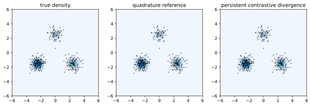
def density_on_grid(energy):
    return jnp.exp(-energy(grid) - log_Z(energy)).reshape(100, 100)

panels = [('true density', jnp.exp(mix.log_prob(grid)).reshape(100, 100)),
          ('quadrature reference', density_on_grid(energy_mle)),
          ('persistent contrastive divergence', density_on_grid(energy_pcd))]
fig, axes = d2l.plt.subplots(1, 3, figsize=(10.5, 3.4))
for ax, (title, dens) in zip(axes, panels):
    ax.contourf(axis, axis, dens.T, levels=12, cmap='Blues')
    ax.scatter(test[:300, 0], test[:300, 1], s=3, c='k', alpha=0.4)
    ax.set_title(title), ax.set_aspect('equal')
fig.tight_layout()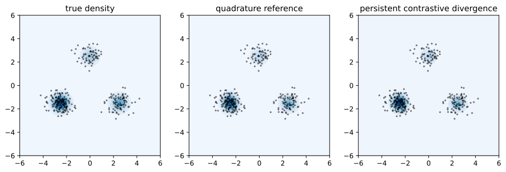
Persistent contrastive divergence recovers the three modes in the right places with approximately the right weights, and by the end of the run its test negative log-likelihood is within a few hundredths of a nat of the quadrature reference. The trace shows how it got there: the value falls over the first checkpoints, then fluctuates between checkpoints and settles only as the learning rate decays. A plausible source of the fluctuation is the negative phase. It is estimated from chains that mix slowly between modes, so the model’s expectation is represented by whatever fraction of chains happens to occupy each mode, and the gradient is biased whenever that fraction differs from the model’s own weights; the bias changes as the energy landscape changes, and a fixed learning rate would keep the parameters moving in response. Exercise 5 tests this explanation. The result took sixty thousand Metropolis–Hastings steps for each of the \(1024\) chains, about sixty million proposals in two dimensions. For images, where each step of a gradient-based sampler costs a forward and a backward pass of a deep network, the same strategy is possible but expensive, and the learned model is sensitive to the settings of the sampler, such as its step size (Du and Mordatch 2019).
Maximum likelihood requires the model’s own samples because its gradient contains the model’s expectation. An objective whose gradient involves only data would remove the inner sampling loop entirely. The score of the next section provides such an objective.
17.2.5 Summary
The gradient of the log-partition function is minus the model’s expected energy gradient, so the maximum-likelihood gradient of an energy-based model is the model expectation minus the data expectation of \(\nabla_{\boldsymbol{\theta}} E_{\boldsymbol{\theta}}\). The update lowers the energy at data and raises it at model samples, and it needs samples rather than the normalizer. In two dimensions the identity was verified against quadrature, with Monte Carlo error falling as \(1 / \sqrt{n}\).
Markov chain Monte Carlo supplies the samples. A kernel that satisfies detailed balance with respect to \(p_{\boldsymbol{\theta}}\) leaves it stationary, and Metropolis–Hastings builds such a kernel from any proposal using only energy differences. Its step size trades acceptance against mixing: on the running example, small proposals get the within-mode spread right but not the weights between modes, while proposals large enough to cross the gaps are rarely accepted but, when accepted, move chains between modes. Contrastive divergence shortens the chains by starting them at data, and persistent contrastive divergence reuses chains across updates. The persistent variant fitted the mixture to within a few hundredths of a nat of the quadrature reference once the learning rate had decayed, at the cost of a sampling loop inside every update and a bias that depends on how well that loop mixes.
17.2.6 Exercises
- The gradient of the normalizer. Repeat the derivation of Equation 17.2.2 for a discrete model \(p_{\boldsymbol{\theta}}(x) = \exp(-E_{\boldsymbol{\theta}}(x)) / Z(\boldsymbol{\theta})\) over a finite set, replacing the integral by a sum. Then specialize to a Gaussian written as an exponential family with sufficient statistics \((x, x^2)\), and verify that setting Equation 17.2.3 to zero matches the first two moments of the data.
- Detailed balance for rejected moves. The proof in the text treated proposals \(\mathbf{x}' \neq \mathbf{x}\). Write the full transition kernel of Metropolis–Hastings, including the probability of remaining at \(\mathbf{x}\), and show that Equation 17.2.4 holds for \(\mathbf{x}' = \mathbf{x}\) trivially. Then show that Gibbs sampling, viewed as a proposal that draws one coordinate from its conditional, has acceptance probability exactly one under Equation 17.2.5.
- [code] Acceptance and dimension. Run the random-walk sampler on a standard Gaussian target in \(d = 2, 8, 32, 128\) dimensions with a fixed step size, and record the acceptance rate. Then find, for each \(d\), the step size that gives an acceptance rate near \(0.25\), and plot it against \(d\) on logarithmic axes. What power law do you observe, and what does it imply for the number of steps needed to move a distance of order one?
- [code] Contrastive divergence with short chains. Train the energy network with chains initialized at the minibatch and run for \(k = 1\) Metropolis–Hastings steps, the original contrastive divergence. Compare the test negative log-likelihood and the learned density with the persistent run. Where does the \(k = 1\) model place spurious probability mass, and why does starting the chains at data make this failure likely?
- [code] The learning-rate schedule. Repeat the persistent run with a constant learning rate of \(2 \times 10^{-3}\) and record the test negative log-likelihood every \(250\) steps. Relate the fluctuations to the mode weights of the persistent chains at the same checkpoints. Does averaging the parameters over the last thousand steps recover the quality of the decayed run?
- [code] An energy-based classifier. Train the energy network as a conditional model \(E_{\boldsymbol{\theta}}(\mathbf{x}, y)\) with \(y\) the index of the component that generated each training point, which the sampler in
GaussianMixture.samplecan be modified to return. Because \(y\) takes three values, the normalizer over \(y\) for fixed \(\mathbf{x}\) is a sum of three terms and needs no sampling. Train by maximum likelihood of \(p(y \mid \mathbf{x})\), report the test accuracy, and explain which quantity this model cannot provide that the unconditional model can. - [code] Mode switches. Rerun the step-size experiment and, for each of the three proposal scales, count how often a chain’s nearest component mean changes during the run, and record the mode weights after \(200\), \(1000\), and \(2000\) steps. Which scale reaches the true weights first, and how does the answer square with its acceptance rate?