%matplotlib inline
from d2l import torch as d2l
import torch17.5 Sampling with Langevin Dynamics
A learned score is a vector field that points toward the data. To turn it into samples, follow it. Gradient ascent on \(\log p\) would climb to a mode and stop there; adding the right amount of noise at each step turns the climb into a Markov chain whose stationary distribution approaches \(p\) as the step size shrinks. This sampler, Langevin dynamics, needs nothing but the score, so it applies to the models of the last two sections directly. This section defines it, tests it on the running example with the true score and with learned scores, and identifies two ways in which it fails: the chain does not move between separated modes, and the learned score is unreliable where the data are absent. Gaussian smoothing addresses both at a price, which motivates the multi-scale approach of the next section. The presentation follows lecture 12 of Kuleshov (2023) .
%matplotlib inline
from d2l import jax as d2l
import jax
from jax import numpy as jnp
from flax import nnx
import optax
17.5.1 The Langevin Update
Langevin dynamics is the Markov chain
\[ \mathbf{x}_{k+1} = \mathbf{x}_k + \frac{\alpha}{2}\, \nabla_{\mathbf{x}} \log p(\mathbf{x}_k) + \sqrt{\alpha}\, \boldsymbol{\xi}_k, \qquad \boldsymbol{\xi}_k \sim \mathcal{N}(\mathbf{0}, I), \tag{17.5.1}\]
started from an arbitrary initial state \(\mathbf{x}_0\) (here the subscript counts Langevin steps) and run with a step size \(\alpha > 0\). Each step is a gradient ascent step on \(\log p\) with step size \(\alpha / 2\) followed by a Gaussian perturbation of variance \(\alpha\). The gradient step concentrates the chain where the density is high; the noise keeps it from collapsing to a mode, and the balance between the two spreads the chains in proportion to the density. The ratio between the two makes \(p\) the target: the update is the Euler–Maruyama discretization (Section 29.2.3.2) of the stochastic differential equation \(d\mathbf{X} = \tfrac12 \nabla \log p(\mathbf{X})\, dt + d\mathbf{W}\), and Section 29.4 proves from the Fokker–Planck equation that \(p\) is a stationary density of this equation (Equation 29.4.9). Under mild conditions the continuous-time process converges to \(p\) from any starting point (Roberts and Tweedie 1996). The discrete chain with a fixed \(\alpha\) converges instead to a distribution that differs from \(p\) by a discretization error, which vanishes as \(\alpha \to 0\) with the number of steps growing correspondingly (Durmus and Moulines 2017), and for targets whose tails are lighter than Gaussian it need not converge at all even though the diffusion does (Roberts and Tweedie 1996). The latter paper also analyzes the Metropolis-adjusted variant, which treats the Langevin move as the proposal of a Metropolis–Hastings step and accepts or rejects it, which removes the discretization bias at the cost of an acceptance test. Score-based models use the unadjusted chain Equation 17.5.1, because it needs the score and nothing else.
The chain is a gradient-informed relative of the random walk of Section 17.2. Where Metropolis–Hastings proposed a blind step and corrected it by an acceptance test, Langevin dynamics takes a step that already points toward higher density. For an energy-based model the score is \(-\nabla E_{\boldsymbol{\theta}}\), so the chain runs on the energy alone. For a score model, substitute \(\mathbf{s}_{\boldsymbol{\theta}}\) for the score in Equation 17.5.1; the chain then samples approximately from \(p\), to the extent that \(\mathbf{s}_{\boldsymbol{\theta}}\) approximates its score. This is the basic generative procedure of Song and Ermon (2019), who then anneal it over noise levels as Section 17.6 describes: estimate the score by score matching, then sample by Langevin dynamics.
The implementation runs many chains in parallel, one per row, and returns their final states. The helper reports the statistics that the running example lets us check: the fraction of chains that end nearest to each component mean, which should match the weights \(0.5\), \(0.3\), \(0.2\); the mean squared distance to that mean over chains that lie within three standard deviations of it; and the fraction of stray chains that end more than three standard deviations from every mean. Exact samples of the mixture do not give a spread of \(2 \times 0.25 = 0.5\) and a stray fraction of zero under this statistic: the truncation lowers the spread to \(0.47\), and the tail of a two-dimensional Gaussian beyond three standard deviations holds a fraction \(e^{-9/2} \approx 0.011\) of its mass. The cells therefore print the statistic of the training sample as the target.
torch.manual_seed(0)
mix = d2l.GaussianMixture(means=[[-2.5, -1.5], [2.5, -1.5], [0.0, 2.5]],
                          weights=[0.5, 0.3, 0.2], std=0.5)
data = mix.sample(2000)

def langevin(score, x, steps, step_size):
    """Unadjusted Langevin dynamics, one chain per row of x."""
    with torch.no_grad():
        for _ in range(steps):
            x = (x + 0.5 * step_size * score(x)
                 + step_size ** 0.5 * torch.randn_like(x))
    return x

def summarize(x):
    """Mode weights, within-mode spread, and the fraction of stray chains."""
    d2 = ((x[:, None, :] - mix.means[None]) ** 2).sum(-1)
    weights = [round(w, 3) for w in
               (torch.bincount(d2.argmin(1), minlength=3) / len(x)).tolist()]
    nearest = d2.min(1).values
    inside = nearest < (3 * mix.std) ** 2
    return (f'mode weights {weights}, spread {nearest[inside].mean():.2f}, '
            f'stray {1 - inside.float().mean():.3f}')
key = jax.random.PRNGKey(0)
mix = d2l.GaussianMixture(means=[[-2.5, -1.5], [2.5, -1.5], [0.0, 2.5]],
weights=[0.5, 0.3, 0.2], std=0.5)
key, subkey = jax.random.split(key)
data = mix.sample(subkey, 2000)
@nnx.jit
def langevin_step(score, x, key, step_size):
return (x + 0.5 * step_size * score(x)
+ step_size ** 0.5 * jax.random.normal(key, x.shape))
def langevin(score, x, key, steps, step_size):
"""Unadjusted Langevin dynamics, one chain per row of x."""
for _ in range(steps):
key, subkey = jax.random.split(key)
x = langevin_step(score, x, subkey, step_size)
return x
def summarize(x):
"""Mode weights, within-mode spread, and the fraction of stray chains."""
d2 = ((x[:, None, :] - mix.means[None]) ** 2).sum(-1)
weights = [round(float(w), 3) for w in
jnp.bincount(d2.argmin(1), length=3) / len(x)]
nearest = d2.min(1)
inside = nearest < (3 * mix.std) ** 2
return (f'mode weights {weights}, spread {nearest[inside].mean():.2f}, '
f'stray {1 - inside.mean():.3f}')
class TrueScore(nnx.Module): # the closed-form score as a jittable module
def __init__(self, sigma=0.0):
self.sigma = sigma
def __call__(self, x):
return mix.score(x, sigma=self.sigma)17.5.2 Two Failures on the Running Example
17.5.2.1 Sampling with the True Score
The first experiment removes all estimation error: the chain uses the exact score of the mixture. Two thousand chains start from a broad Gaussian centered at the origin and run with step size \(0.05\) for two hundred and then two thousand steps. A third run starts every chain inside the first mode.
torch.manual_seed(1)
x_init = 3 * torch.randn(2000, 2)
print(f'target (2000 samples of the mixture): {summarize(data)}')
for steps in (200, 2000):
    print(f'true score, {steps:>4d} steps:   '
          f'{summarize(langevin(mix.score, x_init, steps, 0.05))}')
x_one = mix.means[0] + mix.std * torch.randn(2000, 2)
print(f'true score, start in mode 1: '
      f'{summarize(langevin(mix.score, x_one, 2000, 0.05))}')
target (2000 samples of the mixture): mode weights [0.5, 0.317, 0.183], spread 0.49, stray 0.012
true score, 200 steps: mode weights [0.319, 0.317, 0.364], spread 0.49, stray 0.011
true score, 2000 steps: mode weights [0.322, 0.313, 0.364], spread 0.50, stray 0.014
true score, start in mode 1: mode weights [0.998, 0.001, 0.001], spread 0.49, stray 0.015key, k1, k2 = jax.random.split(key, 3)
x_init = 3 * jax.random.normal(k1, (2000, 2))
true_score = TrueScore()
print(f'target (2000 samples of the mixture): {summarize(data)}')
for steps in (200, 2000):
key, subkey = jax.random.split(key)
print(f'true score, {steps:>4d} steps: '
f'{summarize(langevin(true_score, x_init, subkey, steps, 0.05))}')
x_one = mix.means[0] + mix.std * jax.random.normal(k2, (2000, 2))
key, subkey = jax.random.split(key)
print(f'true score, start in mode 1: '
f'{summarize(langevin(true_score, x_one, subkey, 2000, 0.05))}')target (2000 samples of the mixture): mode weights [0.517, 0.296, 0.187], spread 0.46, stray 0.011
true score, 200 steps: mode weights [0.318, 0.325, 0.358], spread 0.48, stray 0.019
true score, 2000 steps: mode weights [0.32, 0.327, 0.354], spread 0.51, stray 0.020
true score, start in mode 1: mode weights [0.999, 0.001, 0.001], spread 0.50, stray 0.012Within each mode the chain is correct: the spread matches the target’s to within the discretization bias, and the stray fraction is close to that of exact samples, one to two percent. Between modes it is stuck. After two hundred steps the three modes hold roughly equal fractions of the chains, which is where the broad initialization sent them, and after ten times as many steps the fractions are unchanged. Chains started inside one mode remain there. Nothing is wrong with the score: given enough steps, the chain would reach the right weights up to its discretization bias. The two lower modes are ten standard deviations apart and the upper one about nine and a half from each, and to cross from one to another a chain must climb against the gradient to the floor of the valley between them, about five standard deviations from either mode, where the density is smaller than at the modes by a factor between about \(e^{-10}\) and \(e^{-12}\). The noise term occasionally pushes a chain outward, but the gradient term pulls it back long before it reaches the valley. The expected waiting time for a crossing exceeds the run by orders of magnitude (Exercise 2 estimates it), so the weights the chain reports are the weights of its initialization. This slow mixing is the same defect that the random-walk sampler showed, and the gradient does not cure it (Song and Ermon 2019). The trajectories below show the mechanism: chains started far out fall quickly into whichever basin they begin in and then wander inside it.
torch.manual_seed(2)
x, path = 3 * torch.randn(8, 2), []
with torch.no_grad():
    for _ in range(300):
        path.append(x)
        x = x + 0.5 * 0.05 * mix.score(x) + 0.05 ** 0.5 * torch.randn_like(x)
path = torch.stack(path)  # (steps, chains, 2)
axis = torch.linspace(-6, 6, 121)
grid = torch.stack(torch.meshgrid(axis, axis, indexing='ij'), -1).reshape(-1, 2)
d2l.set_figsize((4.5, 4.5))
d2l.plt.contourf(axis, axis, torch.exp(mix.log_prob(grid)).reshape(121, 121).T,
                 levels=12, cmap='Blues')
for i in range(8):
    d2l.plt.plot(path[:, i, 0], path[:, i, 1], lw=0.8)
    d2l.plt.plot(path[0, i, 0], path[0, i, 1], 'ko', ms=3)
d2l.plt.xlabel('$x_1$'), d2l.plt.ylabel('$x_2$');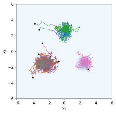
key, subkey = jax.random.split(key)
x, path = 3 * jax.random.normal(subkey, (8, 2)), []
for _ in range(300):
    path.append(x)
    key, subkey = jax.random.split(key)
    x = langevin_step(true_score, x, subkey, 0.05)
path = jnp.stack(path)  # (steps, chains, 2)
axis = jnp.linspace(-6, 6, 121)
grid = jnp.stack(jnp.meshgrid(axis, axis, indexing='ij'), -1).reshape(-1, 2)
d2l.set_figsize((4.5, 4.5))
d2l.plt.contourf(axis, axis, jnp.exp(mix.log_prob(grid)).reshape(121, 121).T,
                 levels=12, cmap='Blues')
for i in range(8):
    d2l.plt.plot(path[:, i, 0], path[:, i, 1], lw=0.8)
    d2l.plt.plot(path[0, i, 0], path[0, i, 1], 'ko', ms=3)
d2l.plt.xlabel('$x_1$'), d2l.plt.ylabel('$x_2$');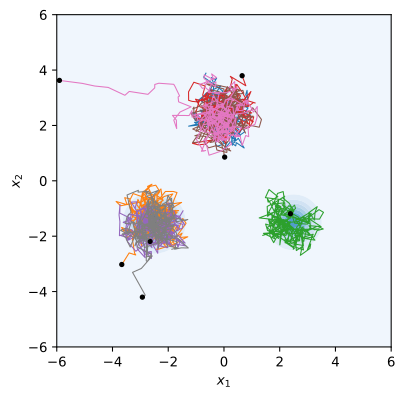
17.5.2.2 Sampling with a Learned Score
A learned score adds a second problem. Section 17.3 measured the relative error of a score matching estimate and found it under ten percent where the data are and ten to twenty percent far below the modes in density. A chain started from noise spends its first steps in those low-density regions. Figure 17.5.1 sketches the situation: inside the region that holds the data, the estimated field agrees with the truth; outside it, the arrows have no reason to be right, and a chain that begins outside is steered by them until it happens to reach the region where the estimate is trustworthy.
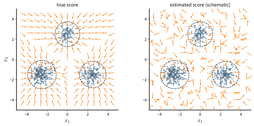
For images the problem is more severe than the sketch suggests. Under the manifold hypothesis the data concentrate near a low-dimensional set, so almost all of pixel space is a low-density region, the score there is undefined or ill-conditioned, and a chain initialized from noise has to traverse this region before any learned estimate becomes reliable (Song and Ermon 2019). In two dimensions the effect is milder, and the experiment measures how much of it survives. We train the score network by sliced score matching, as in Section 17.3, and run the same chains as before.
def sliced_score_matching_loss(score, x):
    x = x.clone().requires_grad_(True)
    v = torch.randn_like(x)
    s = score(x)
    jv = torch.autograd.grad((s * v).sum(), x, create_graph=True)[0]
    return ((v * jv).sum(1) + 0.5 * (s * v).sum(1) ** 2).mean()

def train(loss_fn, steps=2000, lr=1e-3, seed=1):
    torch.manual_seed(seed)
    score = d2l.ScoreNet()
    optimizer = torch.optim.Adam(score.parameters(), lr=lr)
    for step in range(steps):
        x = data[torch.randint(0, len(data), (256,))]
        loss = loss_fn(score, x)
        optimizer.zero_grad(), loss.backward(), optimizer.step()
    return score

score_data = train(sliced_score_matching_loss)
print(f'learned score of the data: '
      f'{summarize(langevin(score_data, x_init, 2000, 0.05))}')
learned score of the data: mode weights [0.396, 0.312, 0.292], spread 0.49, stray 0.027def sliced_score_matching_loss(score, x, v):
f = lambda q: score(q[None])[0]
s, jv = jax.vmap(lambda q, u: jax.jvp(f, (q,), (u,)))(x, v)
return ((v * jv).sum(1) + 0.5 * (s * v).sum(1) ** 2).mean()
@nnx.jit
def sliced_step(score, optimizer, x, v):
loss, grads = nnx.value_and_grad(sliced_score_matching_loss)(score, x, v)
optimizer.update(score, grads)
return loss
def train(step_fn, key, steps=2000, lr=1e-3, seed=1):
score = d2l.ScoreNet(rngs=nnx.Rngs(seed))
optimizer = nnx.Optimizer(score, optax.adam(lr), wrt=nnx.Param)
for step in range(steps):
key, k1, k2 = jax.random.split(key, 3)
x = data[jax.random.randint(k1, (256,), 0, len(data))]
step_fn(score, optimizer, x, jax.random.normal(k2, x.shape))
return score
key, k1, k2 = jax.random.split(key, 3)
score_data = train(sliced_step, k1)
print(f'learned score of the data: '
f'{summarize(langevin(score_data, x_init, k2, 2000, 0.05))}')learned score of the data: mode weights [0.373, 0.318, 0.31], spread 0.47, stray 0.018The learned score reproduces the within-mode spread, and its mode weights are still wrong: they are set by where the field steers the chains from their initialization, not by the data, and they differ from the true field’s because the two fields steer differently far from the modes. The stray fraction, a few percent, is comparable to the exact field’s: almost every chain still reaches a basin, so along the paths the chains take the learned field points roughly inward. This experiment cannot separate estimation error from the one percent of strays that exact samples have. The image case, in which the region where the estimate is unreliable is almost all of pixel space, is the one that the next section addresses.
17.5.3 Gaussian Smoothing and Its Price
Both failures share a cause: the empty regions between and around the modes. Perturbing the data with Gaussian noise fills them. Section 17.4 showed that the score of the perturbed distribution \(p_\sigma\) can be learned everywhere the noisy samples reach, and that at a large \(\sigma\) the learned field is organized across the whole plotted region. Between the modes of \(p_\sigma\) the density is no longer negligible, so a chain can cross. The experiment trains scores of \(p_\sigma\) by denoising score matching at two noise levels and runs the chains on each, together with the true score of \(p_\sigma\) for comparison. The reference statistics now describe the perturbed distribution, whose components have variance \(0.25 + \sigma^2\) per coordinate; the cells print the statistic of exact samples of \(p_\sigma\) as the target. Because the statistic keeps only chains within three data standard deviations of a mean, it truncates the wider distribution, and at \(\sigma = 1\) a large fraction of exact samples counts as stray.
def denoising_loss(score, x, sigma):
    eps = torch.randn_like(x)
    return 0.5 * ((score(x + sigma * eps) + eps / sigma) ** 2).sum(1).mean()

samples = {}
for sigma in (0.3, 1.0):
    print(f'sigma = {sigma}: target (p_sigma samples): '
          f'{summarize(data + sigma * torch.randn_like(data))}')
    score_sigma = train(lambda s, x: denoising_loss(s, x, sigma))
    samples[sigma] = langevin(score_sigma, x_init, 2000, 0.05)
    print(f'sigma = {sigma}: learned score of p_sigma: {summarize(samples[sigma])}')
    smoothed = lambda x: mix.score(x, sigma=sigma)
    print(f'sigma = {sigma}: true score of p_sigma:    '
          f'{summarize(langevin(smoothed, x_init, 2000, 0.05))}')
sigma = 0.3: target (p_sigma samples): mode weights [0.5, 0.317, 0.183], spread 0.60, stray 0.041
sigma = 0.3: learned score of p_sigma: mode weights [0.477, 0.24, 0.283], spread 0.60, stray 0.057
sigma = 0.3: true score of p_sigma: mode weights [0.34, 0.322, 0.338], spread 0.60, stray 0.047
sigma = 1.0: target (p_sigma samples): mode weights [0.491, 0.318, 0.191], spread 0.95, stray 0.386
sigma = 1.0: learned score of p_sigma: mode weights [0.513, 0.288, 0.199], spread 0.99, stray 0.409
sigma = 1.0: true score of p_sigma: mode weights [0.491, 0.301, 0.208], spread 0.97, stray 0.430def denoising_loss(score, x, eps, sigma):
return 0.5 * ((score(x + sigma * eps) + eps / sigma) ** 2).sum(1).mean()
@nnx.jit
def denoising_step(score, optimizer, x, eps, sigma):
loss, grads = nnx.value_and_grad(denoising_loss)(score, x, eps, sigma)
optimizer.update(score, grads)
return loss
samples = {}
for sigma in (0.3, 1.0):
key, k1, k2, k3, k4 = jax.random.split(key, 5)
print(f'sigma = {sigma}: target (p_sigma samples): '
f'{summarize(data + sigma * jax.random.normal(k4, data.shape))}')
step_fn = lambda s, o, x, e: denoising_step(s, o, x, e, sigma)
score_sigma = train(step_fn, k1)
samples[sigma] = langevin(score_sigma, x_init, k2, 2000, 0.05)
print(f'sigma = {sigma}: learned score of p_sigma: {summarize(samples[sigma])}')
print(f'sigma = {sigma}: true score of p_sigma: '
f'{summarize(langevin(TrueScore(sigma), x_init, k3, 2000, 0.05))}')sigma = 0.3: target (p_sigma samples): mode weights [0.517, 0.296, 0.187], spread 0.60, stray 0.034
sigma = 0.3: learned score of p_sigma: mode weights [0.405, 0.339, 0.257], spread 0.57, stray 0.036
sigma = 0.3: true score of p_sigma: mode weights [0.339, 0.335, 0.327], spread 0.59, stray 0.053
sigma = 1.0: target (p_sigma samples): mode weights [0.512, 0.291, 0.198], spread 0.95, stray 0.412
sigma = 1.0: learned score of p_sigma: mode weights [0.527, 0.314, 0.16], spread 0.94, stray 0.396
sigma = 1.0: true score of p_sigma: mode weights [0.47, 0.32, 0.211], spread 0.99, stray 0.411At \(\sigma = 1\) the chains mix: the mode weights come out near \(0.5\), \(0.3\), \(0.2\) with the learned score and with the true one, because the perturbed density has no deep valleys left for the chain to be trapped by. The samples, however, are samples of \(p_\sigma\), whose components have five times the variance of the data’s: even the truncated spread doubles, and about forty percent of the chains end beyond three data standard deviations from every mean, as the target line for \(p_\sigma\) shows. At \(\sigma = 0.3\) the spread matches that of \(p_\sigma\), about a quarter above the data’s, but the valleys are still deep enough that the weights remain wrong. The panels compare the two sets of samples with the data.
fig, axes = d2l.plt.subplots(1, 3, figsize=(10.5, 3.6))
panels = [('data', data), ('samples, sigma = 0.3', samples[0.3]),
          ('samples, sigma = 1.0', samples[1.0])]
for ax, (title, pts) in zip(axes, panels):
    ax.scatter(pts[:1000, 0], pts[:1000, 1], s=3)
    ax.set_xlim(-6, 6), ax.set_ylim(-6, 6), ax.set_aspect('equal')
    ax.set_title(title)
fig.tight_layout()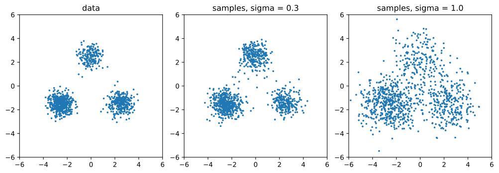
fig, axes = d2l.plt.subplots(1, 3, figsize=(10.5, 3.6))
panels = [('data', data), ('samples, sigma = 0.3', samples[0.3]),
          ('samples, sigma = 1.0', samples[1.0])]
for ax, (title, pts) in zip(axes, panels):
    ax.scatter(pts[:1000, 0], pts[:1000, 1], s=3)
    ax.set_xlim(-6, 6), ax.set_ylim(-6, 6), ax.set_aspect('equal')
    ax.set_title(title)
fig.tight_layout()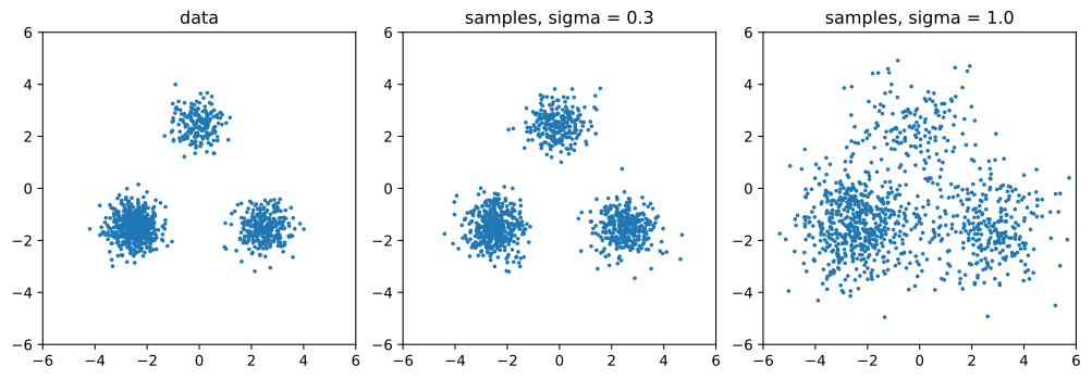
The trade-off is now explicit. A large noise level gives a chain that mixes and a score that is reliable wherever the noisy data reach, at the cost of sampling a blurred version of the data. A small noise level preserves the data but restores both failures, so no single \(\sigma\) serves. The resolution is to use several: run the chain at a large noise level until it has found the right proportions, then decrease the noise and continue, so that each level hands the next a starting point that is likely to lie where the finer score is well estimated. Making this idea precise requires a score model conditioned on the noise level, which is the subject of the next section.
17.5.4 Summary
Langevin dynamics Equation 17.5.1 samples from a density using only its score: a gradient step with step size \(\alpha / 2\) followed by Gaussian noise of variance \(\alpha\) leaves \(p\) stationary in the continuous-time limit, and the discretized chain approaches \(p\) up to a discretization bias that vanishes with the step size. Substituting a learned score gives a generative model without a normalizer, a Markov chain inside training, or a second network.
On the running example the chain reproduced each mode’s spread to within the discretization bias but almost never moved between them, so the mode weights reflected the initialization after two thousand steps as after two hundred. With a learned score the same happened, with mode weights that were wrong in a different way and a stray fraction comparable to that of exact samples. Smoothing the data with noise of scale \(\sigma = 1\) restored approximately correct mode weights with both the learned and the true score, because the perturbed density has no deep valleys, but the samples were those of the blurred distribution. Sharp samples and correct proportions require different noise levels, and the next section uses a ladder of them.
17.5.5 Exercises
- Stationarity in one dimension. For \(p(x) \propto e^{-x^2 / 2}\), the Langevin update Equation 17.5.1 is linear: \(x_{k+1} = (1 - \alpha / 2) x_k + \sqrt{\alpha}\, \xi_k\). For \(0 < \alpha < 4\), compute the variance of the stationary distribution of this chain as a function of \(\alpha\), show that it exceeds \(1\), and expand the excess to first order in \(\alpha\). This is the discretization bias of the unadjusted chain in the simplest case.
- Escaping a mode. Model the valley between two modes of the running example by a one-dimensional density \(p(x) \propto e^{-U(x)}\) with a barrier of height \(\Delta U\) between two wells. Using the fact that the stationary density at the barrier top is smaller than at the well bottom by a factor of \(e^{\Delta U}\), argue that, in the limit of small \(\alpha\), the expected number of steps before a crossing grows like \(e^{\Delta U}\), up to a factor that depends on \(\alpha\) and on the curvature of \(U\) at the well bottom and at the barrier top. Estimate \(\Delta U\) for two Gaussian modes of standard deviation \(0.5\) whose means are \(5\) apart, and compare the resulting waiting time with the two thousand steps of the experiment.
- [code] Step size. Repeat the true-score experiment with step sizes \(0.005\), \(0.05\), and \(0.5\) for two thousand steps each, and report the within-mode spread and the stray fraction. Explain the two failure directions: what happens to the spread when \(\alpha\) is large, and what happens to the distance traveled from the initialization when \(\alpha\) is small?
- [code] Metropolis adjustment. Add an acceptance test to the Langevin move, treating Equation 17.5.1 as the proposal \(Q(\mathbf{x}' \mid \mathbf{x}) = \mathcal{N}(\mathbf{x} + \tfrac{\alpha}{2} \nabla \log p(\mathbf{x}),\, \alpha I)\) in Equation 17.2.5; note that this proposal is not symmetric. Verify that with the true score the within-mode spread becomes exact even at a large step size, and measure the acceptance rate as a function of \(\alpha\).
- [code] Fewer data. Train the sliced score matching model on \(200\) training points instead of \(2000\) and repeat the learned-score sampling run. How do the stray fraction and the within-mode spread change, and which of the two failures discussed in the section does the change reflect?
- [code] A denoising step at the end. For the run at \(\sigma = 1\), apply Tweedie’s formula Equation 17.4.4 once to the final samples, moving each by \(\sigma^2\) times the learned score. Report the spread and the mode weights of the result and compare them with the data. Which aspect of the blur does one denoising step remove, and which does it not?