%matplotlib inline
from d2l import torch as d2l
import math
import torch
from torch import nn17.1 The Limits of GANs and Energy-Based Models
Two families of generative models leave the network that defines them nearly free. Generative adversarial networks (Chapter 16) place no architectural restriction on the generator because they never evaluate its density: a second network compares samples with data and supplies the training signal. Energy-based models place no architectural restriction on the network either, but for the opposite reason: they do define a density, through an unnormalized function whose integral is left implicit and only has to be finite. This section records what each family pays for its freedom. The adversarial game pays in optimization: its dynamics need not converge, its gradients can vanish, and it can settle on a fraction of the data. The energy-based model pays in computation: its normalizing constant is an integral over the whole input space, and the rest of the chapter is organized around avoiding it. The presentation follows lectures 10 and 11 of Kuleshov (2023) .
%matplotlib inline
from d2l import jax as d2l
import math
import jax
from jax import numpy as jnp
from flax import nnx
17.1.1 What Adversarial Training Leaves Unsolved
A generative adversarial network trains a generator \(G\) and a discriminator \(D\) on the value function of Equation 16.1.1, the generator minimizing and the discriminator maximizing. Section 16.1 showed that at the discriminator’s best response the generator minimizes the Jensen–Shannon divergence between its distribution and the data. The fixed point is the right one. Four difficulties remain, and none of them concerns the fixed point itself (Goodfellow 2016; Kuleshov 2023).
The first difficulty is that the objective is a game rather than a loss. Simultaneous gradient steps on a minimax objective can circle the equilibrium or spiral away from it instead of approaching it, even in the two-parameter Dirac-GAN of Section 16.4. In that example, a zero-centered gradient penalty, which the original formulation lacks, makes the equilibrium locally attracting.
The second difficulty is the generator’s gradient. When the discriminator separates real and generated samples confidently, the saturating generator loss assigns each generated sample a weight, the factor in Equation 16.1.5 that multiplies its contribution to the update, that is near zero, and the gradient vanishes as the discriminator approaches the optimum. The non-saturating loss keeps the weight from vanishing but changes the objective. When both distributions have densities and the discriminator is optimal, the expected gradient of the non-saturating loss is the gradient of \(\mathrm{KL}(p_g \,\|\, p_{\textrm{data}}) - 2\, \mathrm{JS}(p_g, p_{\textrm{data}})\), with \(p_g\) the generated distribution (Arjovsky and Bottou 2017). This difference equals \(2\, \mathrm{KL}(m \,\|\, p_{\textrm{data}})\), where \(m = (p_g + p_{\textrm{data}}) / 2\). That divergence is zero only at \(p_g = p_{\textrm{data}}\), so the fixed point is unchanged; like the reverse divergence \(\mathrm{KL}(p_g \,\|\, p_{\textrm{data}})\) (Section 28.2.2.2), however, it penalizes generated samples where the data have little mass far more heavily than missing modes. Worse, if the error of an imperfect discriminator is modeled as independent Gaussian noise at every point, each coordinate of the non-saturating update follows a Cauchy distribution, which has neither a finite mean nor a finite variance (Arjovsky and Bottou 2017). Both the vanishing of the saturating gradient and this instability are derived for the case in which a perfect discriminator exists. That case is typical when the two distributions lie on low-dimensional sets: a generator’s samples lie in a set whose dimension is at most that of its latent space, and real images are believed to concentrate near such a set (Arjovsky and Bottou 2017).
The third difficulty is mode collapse. The generator can obtain a high discriminator score by concentrating on a few regions of the data distribution, and the finite-sample game contains minima at which whole modes are missing (Section 16.3; the mode-coverage experiment of Section 16.4). The remedies are largely empirical: feature matching, minibatch discrimination, one-sided label smoothing, and changes to normalization and architecture (Salimans et al. 2016; Kuleshov 2023).
The fourth difficulty is that the model provides no density. Held-out likelihood cannot be reported, two trained generators cannot be compared by the probability they assign to a test set, and anomalies cannot be scored by their probability. Evaluation relies on feature-space statistics of samples, whose limitations Section 16.5 examined. A separate restriction, not a difficulty of the game itself, is that the generator is trained through the gradient of the discriminator with respect to the generated sample, so the basic formulation requires continuous data.
Some of these difficulties have partial answers within the adversarial framework, and Chapter 16 developed them. This chapter takes a different route. It returns to models with a density, removes the architectural constraints that made likelihood tractable, and then asks how such a model can be trained at all.
17.1.2 Energy-Based Models
17.1.2.1 The Normalization Constraint
A probability density must satisfy two conditions: \(p(\mathbf{x}) \geq 0\) for every \(\mathbf{x}\), and \(\int p(\mathbf{x})\, d\mathbf{x} = 1\). Nonnegativity is easy to enforce. For any network \(f_{\boldsymbol{\theta}}\), the functions \(f_{\boldsymbol{\theta}}(\mathbf{x})^2\) and \(\exp(f_{\boldsymbol{\theta}}(\mathbf{x}))\) are nonnegative. Neither need integrate to one, and the second condition is the one that gives learning its meaning. Because the total mass is fixed, raising the density on the training points necessarily lowers it elsewhere. A model that could raise its value everywhere would fit the data without learning anything about where the data are not (Kuleshov 2023).
Likelihood-based models satisfy the second condition by construction. An autoregressive model multiplies conditionals, each normalized over its own variable given the preceding ones, and integrating out the variables one at a time, last first, shows that the product integrates to one. A mixture or latent-variable model averages normalized components with weights that sum to one. A normalizing flow pushes a simple density through a bijection and tracks the change of volume through the Jacobian determinant (Section 29.1.5). Each construction has a price. Conditionals must be ordered and masked. A latent-variable model is normalized for free, but its likelihood is itself a sum or an integral over the latent variable, so the sum or integral must be tractable, or the model must be trained through a lower bound on the log-likelihood. Flows must be invertible with a computable determinant.
17.1.2.2 Definition
An energy-based model drops these restrictions. It specifies the density through a scalar function \(E_{\boldsymbol{\theta}}: \mathbb{R}^d \to \mathbb{R}\), the energy, which may be any network that satisfies the integrability condition below, and normalizes explicitly:
\[ p_{\boldsymbol{\theta}}(\mathbf{x}) = \frac{\exp(-E_{\boldsymbol{\theta}}(\mathbf{x}))}{Z(\boldsymbol{\theta})}, \qquad Z(\boldsymbol{\theta}) = \int \exp(-E_{\boldsymbol{\theta}}(\mathbf{x}))\, d\mathbf{x}. \tag{17.1.1}\]
The denominator \(Z(\boldsymbol{\theta})\) is the partition function. Low energy means high density (Figure 17.1.1), and the density is defined whenever the integral is finite, which holds when \(E_{\boldsymbol{\theta}}\) grows fast enough at infinity. A network with bounded activations does not satisfy this requirement on its own, so implementations add a term such as \(\|\mathbf{x}\|^2 / 2\) or restrict the domain. The lecture notation writes \(f_{\boldsymbol{\theta}} = -E_{\boldsymbol{\theta}}\); the sign is a convention and nothing else changes.
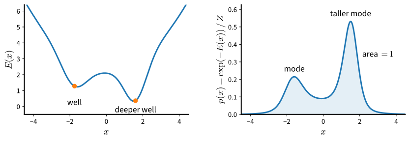
Three reasons make the exponential the natural link between an unconstrained function and a density (Kuleshov 2023). Probabilities of natural data vary over many orders of magnitude, and the logarithm is the scale on which a smooth network can represent such variation. The exponential families of Section 27.2, which include the Gaussian, Bernoulli, and categorical distributions, already have the form Equation 17.1.1 with an energy linear in the parameters. In statistical physics, a system in thermal equilibrium occupies a state of energy \(E\) with probability proportional to \(\exp(-E)\) in suitable units, the Boltzmann distribution, and the name energy comes from this correspondence (LeCun et al. 2006).
The advantage of the definition is its flexibility. Any architecture that produces a scalar can serve as an energy, energies can be added, and adding energies multiplies densities, so a product of experts combines several models into one without renormalizing each factor (Hinton 2002). Most of the disadvantages follow from \(Z(\boldsymbol{\theta})\). Evaluating the likelihood requires it. Its gradient with respect to \(\boldsymbol{\theta}\) appears in every maximum-likelihood update, as Section 17.2 shows. Sampling has no direct algorithm: the model specifies a density rather than a procedure that produces draws, and the Markov chain methods of Section 17.2, which do not need the constant, are slow. A separate limitation is that the model as stated has no latent variables, so it provides no inferred representation of an input, although latent variables can be added.
17.1.2.3 What Can Be Computed Without the Normalizer
Several quantities cancel \(Z(\boldsymbol{\theta})\) and are therefore available from the energy alone. The ratio of two densities is
\[ \frac{p_{\boldsymbol{\theta}}(\mathbf{x})}{p_{\boldsymbol{\theta}}(\mathbf{x}')} = \exp\big(E_{\boldsymbol{\theta}}(\mathbf{x}') - E_{\boldsymbol{\theta}}(\mathbf{x})\big), \]
so comparing two inputs, ranking a set of inputs, or deciding whether a new input is far less probable than typical data all require only differences of energies. Denoising and imputation can be posed as optimization: given a corrupted input, find the nearby \(\mathbf{x}\) of lowest energy, or fill in missing coordinates by minimizing the energy over them. A conditional energy \(E_{\boldsymbol{\theta}}(\mathbf{x}, y)\) over inputs and outputs yields a prediction by minimizing over \(y\), and much of supervised learning can be written in this form (LeCun et al. 2006). The gradient of the log-density with respect to the input, \(\nabla_{\mathbf{x}} \log p_{\boldsymbol{\theta}}(\mathbf{x}) = -\nabla_{\mathbf{x}} E_{\boldsymbol{\theta}}(\mathbf{x})\), is also free of the constant; it is the quantity on which the rest of this chapter is built. What none of these operations provides is a sample from \(p_{\boldsymbol{\theta}}\) or the value of the likelihood.
17.1.2.4 Classical Energy-Based Models
Energy-based models predate deep learning. The Ising model of ferromagnetism (Ising 1925) assigns an energy to a configuration of binary variables that rewards agreement between neighbors. Used as a prior over images, and combined with a term that ties each pixel to a noisy observation, it becomes a Markov random field whose most probable configuration is a denoised image (Geman and Geman 1984; Kuleshov 2023). Boltzmann machines add hidden units with pairwise energies (Ackley et al. 1985); restricting the connections to run between visible and hidden units gives the restricted Boltzmann machine (Smolensky 1986; Hinton 2002), and stacking such layers gives the deep Boltzmann machine (Salakhutdinov and Hinton 2009), an early deep generative model. These models have discrete variables and energies that are quadratic in the variables. The energy-based models of this chapter have continuous inputs and energies given by deep networks, and the difficulty they inherit is the same one: the constant in Equation 17.1.1.
17.1.3 The Cost of the Normalizing Constant
The partition function is a \(d\)-dimensional integral, and the two simplest ways to approximate it, quadrature on a grid and importance sampling from a fixed proposal, both degrade as \(d\) grows. The following experiments measure how quickly.
17.1.3.1 Quadrature
We begin where the integral can be computed. The energy below is a small network with a quadratic term that keeps \(\exp(-E)\) integrable. In one dimension, a grid with spacing \(\Delta\) gives \(Z \approx \Delta \sum_i \exp(-E(x_i))\). Dividing by this sum makes the density sum to one on the grid by construction, which the first printed line checks, and the grid spacing controls how accurately the sum approximates the integral. The ratio of two densities, by contrast, needs no grid at all.
def make_energy(d, seed=0):
    torch.manual_seed(seed)
    net = nn.Sequential(nn.Linear(d, 32), nn.Tanh(), nn.Linear(32, 1))
    nn.init.normal_(net[0].weight, 0, 1.5), nn.init.normal_(net[0].bias, 0, 1.5)
    nn.init.normal_(net[2].weight, 0, 0.4), nn.init.zeros_(net[2].bias)
    # The quadratic term confines the density so that Z is finite
    return lambda x: net(x).squeeze(-1) + 0.5 * (x ** 2).sum(-1)

energy = make_energy(1)
grid = torch.linspace(-6, 6, 1201)[:, None]
dx = float(grid[1, 0] - grid[0, 0])
with torch.no_grad():
    E = energy(grid)
    Z = torch.exp(-E).sum() * dx
    density = torch.exp(-E) / Z
    x0, x1 = torch.tensor([[-1.0]]), torch.tensor([[1.0]])
    ratio = torch.exp(energy(x1) - energy(x0)).item()
print(f'Z = {Z:.4f}; the normalized density integrates to '
      f'{density.sum() * dx:.4f}')
print(f'p(-1)/p(1) from energies alone: {ratio:.4f}; '
      f'from the normalized density: {density[500] / density[700]:.4f}')
fig, axes = d2l.plt.subplots(1, 2, figsize=(8, 3))
axes[0].plot(grid[:, 0], E), axes[0].set_xlabel('x'), axes[0].set_ylabel('E(x)')
axes[1].plot(grid[:, 0], density), axes[1].set_xlabel('x')
axes[1].set_ylabel('p(x) = exp(-E(x)) / Z')
fig.tight_layout()
Z = 7.2918; the normalized density integrates to 1.0000
p(-1)/p(1) from energies alone: 1.8250; from the normalized density: 1.8250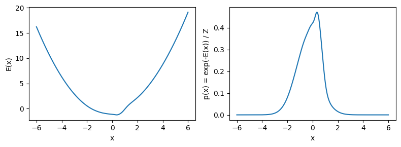
class EnergyNet(nnx.Module):
    def __init__(self, d, rngs):
        self.h = nnx.Linear(d, 32, kernel_init=nnx.initializers.normal(1.5),
                            bias_init=nnx.initializers.normal(1.5), rngs=rngs)
        self.out = nnx.Linear(32, 1, kernel_init=nnx.initializers.normal(0.4),
                              rngs=rngs)

    def __call__(self, x):
        # The quadratic term confines the density so that Z is finite
        return self.out(nnx.tanh(self.h(x)))[..., 0] + 0.5 * (x ** 2).sum(-1)

def make_energy(d, seed=0):
    return EnergyNet(d, nnx.Rngs(seed))

energy = make_energy(1)
grid = jnp.linspace(-6, 6, 1201)[:, None]
dx = float(grid[1, 0] - grid[0, 0])
E = energy(grid)
Z = jnp.exp(-E).sum() * dx
density = jnp.exp(-E) / Z
x0, x1 = jnp.array([[-1.0]]), jnp.array([[1.0]])
ratio = float(jnp.exp(energy(x1) - energy(x0))[0])
print(f'Z = {Z:.4f}; the normalized density integrates to '
      f'{density.sum() * dx:.4f}')
print(f'p(-1)/p(1) from energies alone: {ratio:.4f}; '
      f'from the normalized density: {density[500] / density[700]:.4f}')
fig, axes = d2l.plt.subplots(1, 2, figsize=(8, 3))
axes[0].plot(grid[:, 0], E), axes[0].set_xlabel('x'), axes[0].set_ylabel('E(x)')
axes[1].plot(grid[:, 0], density), axes[1].set_xlabel('x')
axes[1].set_ylabel('p(x) = exp(-E(x)) / Z')
fig.tight_layout()
Z = 10.1219; the normalized density integrates to 1.0000
p(-1)/p(1) from energies alone: 17.8175; from the normalized density: 17.8175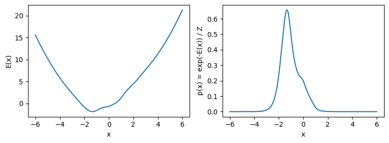
The two ratios agree, as they must, and the quadrature in one dimension costs about a thousand energy evaluations. A grid with \(K\) points per axis in \(d\) dimensions has \(K^d\) points. The next cell repeats the computation for \(d = 1, 2, 3\) with \(K = 64\), using a random energy of the same form for each \(d\), and reports the number of energy evaluations that the normalizer costs. It then prints the count for two larger values of \(d\): ten, and the \(784\) pixels of a Fashion-MNIST image.
K = 64
axis = torch.linspace(-6, 6, K)
for d in (1, 2, 3):
    energy_d = make_energy(d)
    pts = torch.stack(torch.meshgrid(*([axis] * d), indexing='ij'),
                      -1).reshape(-1, d)
    with torch.no_grad():
        log_Z = (torch.logsumexp(-energy_d(pts), 0)
                 + d * math.log(axis[1] - axis[0]))
    print(f'd = {d}: {len(pts):>7d} energy evaluations, log Z = {log_Z:7.3f}')
for d in (10, 784):
    print(f'd = {d}: {K}^{d} = 10^{d * math.log10(K):.0f} energy evaluations')
d = 1: 64 energy evaluations, log Z = 1.987
d = 2: 4096 energy evaluations, log Z = 2.772
d = 3: 262144 energy evaluations, log Z = 3.888
d = 10: 64^10 = 10^18 energy evaluations
d = 784: 64^784 = 10^1416 energy evaluationsK = 64
axis = jnp.linspace(-6, 6, K)
for d in (1, 2, 3):
energy_d = make_energy(d)
pts = jnp.stack(jnp.meshgrid(*([axis] * d), indexing='ij'),
-1).reshape(-1, d)
log_Z = (jax.nn.logsumexp(-energy_d(pts), 0)
+ d * math.log(axis[1] - axis[0]))
print(f'd = {d}: {len(pts):>7d} energy evaluations, log Z = {log_Z:7.3f}')
for d in (10, 784):
print(f'd = {d}: {K}^{d} = 10^{d * math.log10(K):.0f} energy evaluations')d = 1: 64 energy evaluations, log Z = 2.315
d = 2: 4096 energy evaluations, log Z = 3.643
d = 3: 262144 energy evaluations, log Z = 4.184
d = 10: 64^10 = 10^18 energy evaluations
d = 784: 64^784 = 10^1416 energy evaluationsThree dimensions already require a quarter of a million evaluations. At \(d = 10\) the grid has about \(10^{18}\) points, a billion billion, and at \(d = 784\) the exponent exceeds a thousand. Quadrature is a tool for one, two, or three dimensions, which is why this chapter’s running example is two-dimensional: there, and only there, the normalizer of a learned energy can be computed by quadrature as a reference.
17.1.3.2 Monte Carlo Estimates
The alternative to a grid is a random sample. Importance sampling (Section 27.4.2) draws \(\mathbf{x}_1, \ldots, \mathbf{x}_n\) from a proposal density \(q\) that can be sampled and evaluated, and uses the identity
\[ Z(\boldsymbol{\theta}) = \int \frac{\exp(-E_{\boldsymbol{\theta}}(\mathbf{x}))}{q(\mathbf{x})}\, q(\mathbf{x})\, d\mathbf{x} = \mathbb{E}_{\mathbf{x} \sim q}\big[w(\mathbf{x})\big], \qquad w(\mathbf{x}) = \frac{\exp(-E_{\boldsymbol{\theta}}(\mathbf{x}))}{q(\mathbf{x})}, \]
to estimate \(Z\) by the sample mean of the weights \(w(\mathbf{x}_i)\). The estimator is unbiased for every \(n\), provided that \(q\) is positive wherever \(\exp(-E_{\boldsymbol{\theta}})\) is. Its variance is the problem. The variance of a single weight is \(\mathbb{E}_q[w^2] - Z^2 = Z^2 \big( \int p_{\boldsymbol{\theta}}^2 / q - 1 \big)\), and \(\int p_{\boldsymbol{\theta}}^2 / q \geq 1\), with equality only when \(q = p_{\boldsymbol{\theta}}\). When the target and the proposal factorize over coordinates and differ in the same way in every coordinate, this integral is the \(d\)-th power of a one-dimensional factor greater than one, so the relative variance of the weights grows exponentially in \(d\).
A Gaussian example makes the growth exact. Take the target \(E(\mathbf{x}) = \|\mathbf{x} - \mathbf{m}\|^2 / 2\) with \(\mathbf{m}\) the all-ones vector, whose partition function is \(Z = (2\pi)^{d/2}\), and the proposal \(q = \mathcal{N}(\mathbf{0}, I)\). Then \(w / Z = \exp(\mathbf{m}^\top \mathbf{x} - \|\mathbf{m}\|^2 / 2)\), and because \(\mathbf{m}^\top \mathbf{x} \sim \mathcal{N}(0, d)\) under \(q\), the normalized weight is log-normal with \(\mathbb{E}_q[w / Z] = 1\) and \(\mathbb{E}_q[(w / Z)^2] = e^{d}\) (Exercise 4). The relative standard error of the estimate from \(n\) samples is therefore \(\sqrt{(e^{d} - 1) / n}\), exact for every \(d\) and \(n\). The proposal is only one standard deviation from the target in each coordinate. The cell compares this prediction with the estimate itself and with the effective sample size \((\sum_i w_i)^2 / \sum_i w_i^2\), which counts how many of the \(n\) draws carry appreciable weight.
torch.manual_seed(1)
n = 100_000
print(f'{"d":>3} {"estimate / Z":>13} {"predicted rel. std. error":>26} '
      f'{"effective samples":>18}')
for d in (1, 2, 4, 8, 16, 32):
    x = torch.randn(n, d)                      # proposal q = N(0, I)
    log_w = x.sum(1) - d / 2                   # log (w / Z)
    log_sum = torch.logsumexp(log_w, 0)
    estimate = torch.exp(log_sum - math.log(n))
    ess = torch.exp(2 * log_sum - torch.logsumexp(2 * log_w, 0))
    print(f'{d:>3} {estimate:>13.3f} {math.sqrt((math.exp(d) - 1) / n):>26.3g} '
          f'{ess:>18.1f}')
d estimate / Z predicted rel. std. error effective samples
1 0.999 0.00415 37155.5
2 1.017 0.00799 12501.1
4 1.009 0.0232 2620.7
8 1.038 0.173 132.1
16 0.529 9.43 72.3
32 0.081 2.81e+04 11.0key = jax.random.PRNGKey(1)
n = 100_000
print(f'{"d":>3} {"estimate / Z":>13} {"predicted rel. std. error":>26} '
f'{"effective samples":>18}')
for d in (1, 2, 4, 8, 16, 32):
key, subkey = jax.random.split(key)
x = jax.random.normal(subkey, (n, d)) # proposal q = N(0, I)
log_w = x.sum(1) - d / 2 # log (w / Z)
log_sum = jax.nn.logsumexp(log_w, 0)
estimate = jnp.exp(log_sum - math.log(n))
ess = jnp.exp(2 * log_sum - jax.nn.logsumexp(2 * log_w, 0))
print(f'{d:>3} {estimate:>13.3f} {math.sqrt((math.exp(d) - 1) / n):>26.3g} '
f'{ess:>18.1f}') d estimate / Z predicted rel. std. error effective samples
1 1.000 0.00415 37568.7
2 0.997 0.00799 14351.7
4 0.985 0.0232 1425.4
8 1.003 0.173 145.8
16 1.088 9.43 6.0
32 0.079 2.81e+04 10.5Up to \(d = 8\) the estimate is close to one and the predicted error stays below twenty percent. At \(d = 16\) the predicted relative error is several times the quantity being estimated and the effective sample size has dropped to under a hundred draws, so whether a particular run lands near one is a matter of luck rather than evidence. At \(d = 32\) the estimate is typically far below the truth: the weights that would bring the average up to \(Z\) are attached to draws too rare to appear among a hundred thousand samples. The average of the weights is unbiased only because it is occasionally enormous. A hundred thousand proposals from a distribution that is merely one standard deviation off in each coordinate cannot normalize a Gaussian in thirty-two dimensions, and images have hundreds of thousands.
The conclusion is not that \(Z\) is unknowable but that it is expensive in a way that grows with dimension, whether the integral is attacked by grids or by proposals. Every use of an energy-based model that requires the normalizer inherits this cost. The next section makes the requirement precise for maximum likelihood, and identifies the one operation that an update actually needs: samples from the model.
17.1.4 Summary
Adversarial training and energy-based modeling both permit an almost unrestricted network. The adversarial game has the correct fixed point but may not reach it: simultaneous gradient updates can circle the equilibrium or spiral away from it, the saturating generator loss loses its gradient once a perfect discriminator exists and the non-saturating one becomes noisy, the finite-sample game contains mode-dropping minima, and the trained model provides no density to evaluate. An energy-based model defines a density \(\exp(-E_{\boldsymbol{\theta}}) / Z(\boldsymbol{\theta})\) with any energy for which \(\exp(-E_{\boldsymbol{\theta}})\) is integrable, and inherits, in exchange, the partition function. Density ratios, rankings, and energy minimization need no normalizer. Likelihoods do; samples do not, but they require a Markov chain.
Two experiments measured the cost. Quadrature needs \(K^d\) energy evaluations, which passes a quarter of a million at \(d = 3\) and has an exponent above a thousand for a small image. Importance sampling is unbiased but its relative error is \(\sqrt{(e^d - 1) / n}\) in a Gaussian example whose proposal differs from the target by one standard deviation per coordinate, so a hundred thousand draws stop being informative before \(d = 16\). The chapter therefore proceeds without \(Z(\boldsymbol{\theta})\): first by estimating its gradient with samples, then by objectives that do not involve it at all.
17.1.5 Exercises
- Which operations need the normalizer. For an energy-based model Equation 17.1.1, classify each of the following as computable from \(E_{\boldsymbol{\theta}}\) alone or as requiring \(Z(\boldsymbol{\theta})\): the log-likelihood of a test set; the ratio \(p(\mathbf{x}) / p(\mathbf{x}')\); the most probable completion of an image with a missing patch; the probability that a sample falls in a given region; the Kullback–Leibler divergence between two energy-based models with the same energy but different temperatures \(E / \tau\). Justify each answer in one sentence.
- Integrability. Let \(E_{\boldsymbol{\theta}}\) be a multilayer perceptron with ReLU activations and a linear output layer, so that \(E_{\boldsymbol{\theta}}\) is piecewise linear.
- Show that \(\exp(-E_{\boldsymbol{\theta}})\) can fail to be integrable over \(\mathbb{R}^d\), and give a one-dimensional example.
- Show that adding \(\|\mathbf{x}\|^2 / 2\) to any such energy makes the integral finite.
- Does adding \(\|\mathbf{x}\|\) instead always suffice? Give a proof or a counterexample.
- Products of experts. Let \(p_1 \propto \exp(-E_1)\) and \(p_2 \propto \exp(-E_2)\) be two energy-based models on the same space. Show that the model with energy \(E_1 + E_2\) has density proportional to \(p_1 p_2\), and explain why the same construction is not available for two implicit generators in the sense of Section 16.1. Under which condition on \(p_1\) and \(p_2\) is the product concentrated where neither factor alone is?
- The log-normal weight. In the Gaussian example of the text, with target \(\mathcal{N}(\mathbf{m}, I)\) and proposal \(\mathcal{N}(\mathbf{0}, I)\), derive \(w / Z = \exp(\mathbf{m}^\top \mathbf{x} - \|\mathbf{m}\|^2 / 2)\) and show that \(\mathbb{E}_q[w / Z] = 1\) and \(\mathbb{E}_q[(w / Z)^2] = \exp(\|\mathbf{m}\|^2)\), using the moment generating function of a Gaussian. Conclude that the relative standard error of the \(n\)-sample estimate is \(\sqrt{(e^{\|\mathbf{m}\|^2} - 1) / n}\). How many samples are needed for a relative error of \(0.1\) when \(\|\mathbf{m}\|^2 = 20\)?
- [code] A better proposal. Repeat the importance-sampling experiment with the proposal \(\mathcal{N}(\mathbf{m}, I)\), which matches the target exactly, and then with \(\mathcal{N}(\mathbf{m}, 2 I)\), which matches the mean but not the covariance. Derive the relative variance of the weights in the second case as a function of \(d\) and compare it with the measured effective sample size. What does the comparison say about proposals that are broader than the target?
- [code] Quadrature on the running example. Section 17.2 uses a \(100 \times 100\) grid on \([-6, 6]^2\) to normalize a two-dimensional energy. Compute \(\log Z\) for the mixture density defined there, which is normalized by construction, on grids with \(9\), \(13\), \(17\), \(25\), and \(100\) points per axis, in double precision, and report the error of each. At what grid spacing, relative to the component standard deviation, does the quadrature error fall below \(10^{-3}\), and why does the error fall so quickly once the spacing is below the standard deviation?