%matplotlib inline
from d2l import torch as d2l
import math
import torch
from torch import nn17.6 Noise-Conditional Score Networks and Annealed Langevin Dynamics
The previous section ended with a trade-off that no single noise level can resolve: a heavily smoothed distribution lets Langevin dynamics mix and its score be learned wherever the noisy data reach, but its samples are blurred; a lightly smoothed one preserves the data but restores slow mixing and unreliable scores. Song and Ermon (2019) resolve the trade-off by using many noise levels at once. A single network, conditioned on the noise level, learns the score of the perturbed data at every level of a ladder from coarse to fine. Sampling then anneals: it runs Langevin dynamics at the coarsest level, where the chain moves freely, and hands the result to the next level as its starting point, ending at a level so fine that the perturbed distribution is practically the data distribution. This section builds the network and the sampler, verifies on the running example that annealing recovers what a single level could not, and applies the noise-conditional network to images. The presentation follows lecture 12 of Kuleshov (2023) .
%matplotlib inline
from d2l import jax as d2l
import math
import jax
from jax import numpy as jnp
from flax import nnx
import optax
17.6.1 A Ladder of Noise Levels
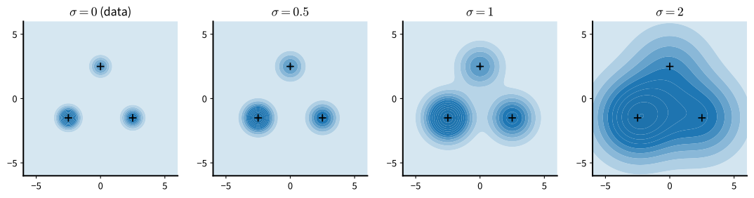
Fix a decreasing sequence of noise levels \(\sigma_1 > \sigma_2 > \cdots > \sigma_L > 0\). The largest is chosen so that \(p_{\sigma_1}\) is close to a single broad Gaussian, with no valleys left between the modes of the data (Song and Ermon (2020) make this precise by taking \(\sigma_1\) about as large as the largest distance between two training points); the smallest is chosen so small that \(p_{\sigma_L}\) is indistinguishable from the data for practical purposes. The levels in between are spaced geometrically, so that each perturbed density differs from its neighbors by a fixed ratio of noise scales. 1 shows what the ladder does to the running example: at \(\sigma = 2\) the three modes have merged into one bump, at \(\sigma = 1\) they are connected through regions of appreciable density, and at \(\sigma = 0.5\) they are nearly separate again.
17.6.1.1 One Network for All Levels
Each level has its own score, so a separate network per level would be one option. A better one is a single network that takes the noise level as an additional input, a noise-conditional score network \(\mathbf{s}_{\boldsymbol{\theta}}(\mathbf{x}, \sigma)\), trained on the denoising objective of Section 17.4 at all levels simultaneously:
\[ \mathcal{L}(\boldsymbol{\theta}) = \frac{1}{L} \sum_{i=1}^{L} \lambda(\sigma_i)\; \mathbb{E}_{\mathbf{x} \sim p,\ \boldsymbol{\epsilon} \sim \mathcal{N}(\mathbf{0}, I)} \left[\, \frac{1}{2} \Big\| \mathbf{s}_{\boldsymbol{\theta}}(\mathbf{x} + \sigma_i \boldsymbol{\epsilon}, \sigma_i) + \frac{\boldsymbol{\epsilon}}{\sigma_i} \Big\|^2 \right]. \tag{17.6.1}\]
A single network also keeps the number of parameters independent of the number of levels, which matters for images: Song and Ermon (2020) use ladders with hundreds of levels. The weights \(\lambda(\sigma_i)\) balance the levels. The regression target \(-\boldsymbol{\epsilon} / \sigma_i\) has squared norm of order \(d / \sigma_i^2\), so without weighting the finest levels would dominate the loss by orders of magnitude. Song and Ermon (2019) choose \(\lambda(\sigma) = \sigma^2\), which turns each level’s term into \(\tfrac12 \mathbb{E}\|\sigma_i \mathbf{s}_{\boldsymbol{\theta}} + \boldsymbol{\epsilon}\|^2\), a regression onto a target of unit variance per coordinate, so that the levels contribute terms of the same order of magnitude instead of being dominated by the finest ones. The same choice suggests the parameterization \(\mathbf{s}_{\boldsymbol{\theta}}(\mathbf{x}, \sigma) = \mathbf{f}_{\boldsymbol{\theta}}(\mathbf{x}, \sigma) / \sigma\), so that the network output \(\mathbf{f}_{\boldsymbol{\theta}}\) is regressed onto \(-\boldsymbol{\epsilon}\) at every level and never has to produce the \(1 / \sigma\) scale itself. Song and Ermon (2020) use the simplest form of this idea, dividing by \(\sigma\) the output of a network that does not see \(\sigma\) at all. With either form the weighted loss is exactly \(\tfrac12 \mathbb{E}\|\mathbf{f}_{\boldsymbol{\theta}} + \boldsymbol{\epsilon}\|^2\) averaged over levels: a noise-prediction loss with a unit-variance target.
For the running example we take ten levels from \(\sigma_1 = 3\) down to \(\sigma_L = 0.05\). The network is the score network of the previous sections with one extra input, \(\log \sigma\), and its output is divided by \(\sigma\).
torch.manual_seed(0)
mix = d2l.GaussianMixture(means=[[-2.5, -1.5], [2.5, -1.5], [0.0, 2.5]],
                          weights=[0.5, 0.3, 0.2], std=0.5)
data, test = mix.sample(2000), mix.sample(2000)
L = 10
sigmas = torch.exp(torch.linspace(math.log(3.0), math.log(0.05), L))
print(f'noise levels: {[round(s, 3) for s in sigmas.tolist()]}')

class NoiseConditionalScoreNet(nn.Module):
    def __init__(self, hidden=128):
        super().__init__()
        self.net = nn.Sequential(nn.Linear(3, hidden), nn.SiLU(),
                                 nn.Linear(hidden, hidden), nn.SiLU(),
                                 nn.Linear(hidden, 2))

    def forward(self, x, sigma):  # sigma has one entry per row of x
        h = torch.cat([x, torch.log(sigma)[:, None]], 1)
        return self.net(h) / sigma[:, None]

def ncsn_loss(score, x):
    sigma = sigmas[torch.randint(0, L, (len(x),))]  # a level per example
    eps = torch.randn_like(x)
    s = score(x + sigma[:, None] * eps, sigma)
    # sigma^2 times the denoising objective at each level
    return 0.5 * (sigma[:, None] ** 2 * (s + eps / sigma[:, None]) ** 2).sum(1).mean()

torch.manual_seed(1)
score = NoiseConditionalScoreNet()
optimizer = torch.optim.Adam(score.parameters(), lr=1e-3)
for step in range(3000):
    loss = ncsn_loss(score, data[torch.randint(0, len(data), (256,))])
    optimizer.zero_grad(), loss.backward(), optimizer.step()
print(f'final training loss: {loss.item():.3f}')
noise levels: [3.0, 1.903, 1.208, 0.766, 0.486, 0.309, 0.196, 0.124, 0.079, 0.05]
final training loss: 0.615key = jax.random.PRNGKey(0)
mix = d2l.GaussianMixture(means=[[-2.5, -1.5], [2.5, -1.5], [0.0, 2.5]],
weights=[0.5, 0.3, 0.2], std=0.5)
key, k1, k2 = jax.random.split(key, 3)
data, test = mix.sample(k1, 2000), mix.sample(k2, 2000)
L = 10
sigmas = jnp.exp(jnp.linspace(math.log(3.0), math.log(0.05), L))
print(f'noise levels: {[round(float(s), 3) for s in sigmas]}')
class NoiseConditionalScoreNet(nnx.Module):
def __init__(self, hidden=128, rngs=None):
self.h1 = nnx.Linear(3, hidden, rngs=rngs)
self.h2 = nnx.Linear(hidden, hidden, rngs=rngs)
self.out = nnx.Linear(hidden, 2, rngs=rngs)
def __call__(self, x, sigma): # sigma has one entry per row of x
h = jnp.concatenate([x, jnp.log(sigma)[:, None]], 1)
return self.out(nnx.silu(self.h2(nnx.silu(self.h1(h))))) / sigma[:, None]
def ncsn_loss(score, x, levels, eps):
sigma = sigmas[levels] # a level per example
s = score(x + sigma[:, None] * eps, sigma)
# sigma^2 times the denoising objective at each level
return 0.5 * (sigma[:, None] ** 2 * (s + eps / sigma[:, None]) ** 2).sum(1).mean()
@nnx.jit
def ncsn_step(score, optimizer, x, levels, eps):
loss, grads = nnx.value_and_grad(ncsn_loss)(score, x, levels, eps)
optimizer.update(score, grads)
return loss
score = NoiseConditionalScoreNet(rngs=nnx.Rngs(1))
optimizer = nnx.Optimizer(score, optax.adam(1e-3), wrt=nnx.Param)
for step in range(3000):
key, k1, k2, k3 = jax.random.split(key, 4)
x = data[jax.random.randint(k1, (256,), 0, len(data))]
loss = ncsn_step(score, optimizer, x, jax.random.randint(k2, (256,), 0, L),
jax.random.normal(k3, x.shape))
print(f'final training loss: {loss:.3f}')noise levels: [3.0, 1.903, 1.208, 0.766, 0.486, 0.309, 0.196, 0.124, 0.079, 0.05]
final training loss: 0.646Because the score of \(p_\sigma\) is known for the running example at every \(\sigma\), the fit can be measured level by level. The cell reports the Fisher divergence at four levels, next to half the mean squared norm of the true score at that level, which sets the scale.
with torch.no_grad():
    print(f'{"sigma":>6} {"Fisher divergence":>18} {"0.5 E||score||^2":>17}')
    for sigma in sigmas[::3]:
        x_noisy = test + sigma * torch.randn_like(test)
        true = mix.score(x_noisy, sigma=sigma.item())
        s = score(x_noisy, torch.full((len(test),), sigma.item()))
        print(f'{sigma:>6.3f} {0.5 * ((s - true) ** 2).sum(1).mean():>18.4f} '
              f'{0.5 * (true ** 2).sum(1).mean():>17.3f}')
sigma Fisher divergence 0.5 E||score||^2
3.000 0.0011 0.079
0.766 0.0412 1.133
0.196 0.1244 3.587
0.050 1.1162 4.086print(f'{"sigma":>6} {"Fisher divergence":>18} {"0.5 E||score||^2":>17}')
for sigma in sigmas[::3]:
key, subkey = jax.random.split(key)
x_noisy = test + sigma * jax.random.normal(subkey, test.shape)
true = mix.score(x_noisy, sigma=float(sigma))
s = score(x_noisy, jnp.full((len(test),), sigma))
print(f'{sigma:>6.3f} {0.5 * ((s - true) ** 2).sum(1).mean():>18.4f} '
f'{0.5 * (true ** 2).sum(1).mean():>17.3f}') sigma Fisher divergence 0.5 E||score||^2
3.000 0.0017 0.076
0.766 0.0296 1.122
0.196 0.1071 3.430
0.050 2.4424 3.950The coarse levels are fitted almost perfectly and the fit degrades toward the finest level, where the target is noisiest and the score is largest; the bias–variance trade-off of Section 17.4 reappears across the rungs of one ladder. The sampler below is designed so that the finest levels have the least to do.
17.6.2 Annealed Langevin Dynamics
Annealed Langevin dynamics (Song and Ermon 2019) runs the Langevin chain of Equation 17.5.1 at each level in turn, from \(\sigma_1\) down to \(\sigma_L\), with the score of that level and a step size proportional to its variance:
\[ \alpha_i = \epsilon\, \frac{\sigma_i^2}{\sigma_L^2}, \qquad \mathbf{x} \leftarrow \mathbf{x} + \frac{\alpha_i}{2}\, \mathbf{s}_{\boldsymbol{\theta}}(\mathbf{x}, \sigma_i) + \sqrt{\alpha_i}\, \boldsymbol{\xi}, \qquad \boldsymbol{\xi} \sim \mathcal{N}(\mathbf{0}, I), \tag{17.6.2}\]
for a fixed number of steps per level (a hundred in the code below), each level starting from the final state of the previous one. The constant \(\epsilon\) follows the notation of Song and Ermon (2019) and is unrelated to the noise vector \(\boldsymbol{\epsilon}\). The chains begin from a broad distribution, such as a uniform or Gaussian cloud covering the data. At the coarsest level the target is nearly Gaussian, and a hundred steps suffice for the chains to sample it approximately; the proportions of the data’s modes form over the next few levels. Each subsequent level sharpens the target slightly; because the chain starts from a sample of the previous, only slightly smoother, distribution, it is likely to begin where the current score is well estimated and to need few steps to adjust (Song and Ermon 2019).
The step size scales with \(\sigma_i^2\) because, for image data, the score of \(p_{\sigma_i}\) grows roughly like \(1 / \sigma_i\) as the level gets finer (Song and Ermon (2019) observe \(\|\mathbf{s}_{\boldsymbol{\theta}}(\mathbf{x}, \sigma)\| \propto 1/\sigma\) for a trained network). The drift \(\alpha_i \mathbf{s}_{\boldsymbol{\theta}} / 2\) and the injected noise \(\sqrt{\alpha_i}\) then both shrink in proportion to \(\sigma_i\), so their ratio, the signal-to-noise ratio of one step, is the same at every level. For the running example this scaling holds only at levels coarser than the components’ standard deviation of \(0.5\): below it the score of \(p_{\sigma_i}\) stops growing (half its mean squared norm in the table above barely changes between \(\sigma = 0.2\) and \(\sigma = 0.05\)), so the finest levels take steps that are small compared with the structure they resolve. At the coarser levels the curvature of \(\log p_{\sigma_i}\) scales as \(1 / \sigma_i^2\), so the contraction per step is level-independent there (Exercise 2). The constant \(\epsilon\) sets the overall scale; we use \(\epsilon = 0.1\, \sigma_L^2\), so that \(\alpha_i = 0.1\, \sigma_i^2\), and the code takes this ratio \(\epsilon / \sigma_L^2\) as its scale argument.
def annealed_langevin(score, x, sigmas, steps_per_level=100, scale=0.1):
    """Langevin dynamics at each level of the ladder, coarse to fine."""
    with torch.no_grad():
        for sigma in sigmas:
            alpha = scale * sigma ** 2  # alpha_i = eps * sigma_i^2 / sigma_L^2
            sigma_vec = torch.full((len(x),), sigma.item())
            for _ in range(steps_per_level):
                x = (x + 0.5 * alpha * score(x, sigma_vec)
                     + alpha ** 0.5 * torch.randn_like(x))
    return x

def summarize(x):
    """Mode weights, within-mode spread, and the fraction of stray chains."""
    d2 = ((x[:, None, :] - mix.means[None]) ** 2).sum(-1)
    weights = [round(w, 3) for w in
               (torch.bincount(d2.argmin(1), minlength=3) / len(x)).tolist()]
    nearest = d2.min(1).values
    inside = nearest < (3 * mix.std) ** 2
    return (f'mode weights {weights}, spread {nearest[inside].mean():.2f}, '
            f'stray {1 - inside.float().mean():.3f}')

torch.manual_seed(2)
x_init = 3 * torch.randn(2000, 2)
print(f'target (2000 samples of the mixture): {summarize(data)}')
for steps in (20, 100):
    x = annealed_langevin(score, x_init, sigmas, steps_per_level=steps)
    print(f'annealed, {steps:>3d} steps per level: {summarize(x)}')
x_single = annealed_langevin(score, x_init, sigmas[-1:], steps_per_level=1000)
print(f'finest level only, 1000 steps:  {summarize(x_single)}')
target (2000 samples of the mixture): mode weights [0.5, 0.317, 0.183], spread 0.49, stray 0.012
annealed, 20 steps per level: mode weights [0.428, 0.314, 0.257], spread 0.75, stray 0.133
annealed, 100 steps per level: mode weights [0.497, 0.298, 0.206], spread 0.54, stray 0.019
finest level only, 1000 steps: mode weights [0.343, 0.317, 0.34], spread 1.04, stray 0.469@nnx.jit
def annealed_step(score, x, key, sigma, alpha):
sigma_vec = jnp.full((len(x),), sigma)
return (x + 0.5 * alpha * score(x, sigma_vec)
+ alpha ** 0.5 * jax.random.normal(key, x.shape))
def annealed_langevin(score, x, key, sigmas, steps_per_level=100, scale=0.1):
"""Langevin dynamics at each level of the ladder, coarse to fine."""
for sigma in sigmas:
alpha = scale * sigma ** 2 # alpha_i = eps * sigma_i^2 / sigma_L^2
for _ in range(steps_per_level):
key, subkey = jax.random.split(key)
x = annealed_step(score, x, subkey, sigma, alpha)
return x
def summarize(x):
"""Mode weights, within-mode spread, and the fraction of stray chains."""
d2 = ((x[:, None, :] - mix.means[None]) ** 2).sum(-1)
weights = [round(float(w), 3) for w in
jnp.bincount(d2.argmin(1), length=3) / len(x)]
nearest = d2.min(1)
inside = nearest < (3 * mix.std) ** 2
return (f'mode weights {weights}, spread {nearest[inside].mean():.2f}, '
f'stray {1 - inside.mean():.3f}')
key, subkey = jax.random.split(key)
x_init = 3 * jax.random.normal(subkey, (2000, 2))
print(f'target (2000 samples of the mixture): {summarize(data)}')
for steps in (20, 100):
key, subkey = jax.random.split(key)
x = annealed_langevin(score, x_init, subkey, sigmas, steps_per_level=steps)
print(f'annealed, {steps:>3d} steps per level: {summarize(x)}')
key, subkey = jax.random.split(key)
x_single = annealed_langevin(score, x_init, subkey, sigmas[-1:],
steps_per_level=1000)
print(f'finest level only, 1000 steps: {summarize(x_single)}')target (2000 samples of the mixture): mode weights [0.517, 0.296, 0.187], spread 0.46, stray 0.011
annealed, 20 steps per level: mode weights [0.439, 0.317, 0.245], spread 0.73, stray 0.137
annealed, 100 steps per level: mode weights [0.487, 0.333, 0.18], spread 0.54, stray 0.023
finest level only, 1000 steps: mode weights [0.385, 0.281, 0.335], spread 1.06, stray 0.491With a hundred steps per level, a thousand network evaluations in all, the annealed chain comes within a few hundredths of the mode weights, with a within-mode spread ten to twenty percent wider than the target’s and about two percent strays against the target’s one: no single-level run in Section 17.5 achieved the three together. Twenty steps per level are not enough at either end of the ladder: the coarse levels do not equilibrate, which leaves the weights off by several hundredths, and the fine levels cannot keep up with the sharpening target, which leaves the spread too large and more than a tenth of the chains stray. Running a thousand steps at the finest level alone, the same budget of network evaluations, fails more severely than any single-level run of Section 17.5: the weights follow the initialization, the spread doubles, and nearly half of the chains are strays. The cause is travel, not estimation. The finest level’s step size \(\alpha_L = 0.1\, \sigma_L^2\) is so small that a thousand steps carry a chain started far out only part of the way to the data, and the exact score of \(p_{\sigma_L}\) gives the same numbers (Exercise 3). The ladder makes the difference: its coarse levels take large steps while the target is still broad. With a hundred steps per level the exact scores of \(p_{\sigma_i}\) give nearly the same statistics as the network (Exercise 3 checks this and compares the two at twenty steps), so most of what remains of the gap to the target at that budget comes from the finite chain rather than from the learned scores.
The panels below follow two thousand chains through the ladder, showing their positions after the levels \(\sigma = 3\), \(0.77\), \(0.2\), and \(0.05\). The cloud contracts from a Gaussian blob to three sharp modes, and the proportions are set at the coarse levels, while the modes are still broad and overlapping; the fine levels only sharpen them.
torch.manual_seed(3)
x, snapshots = x_init.clone(), []
for i in range(L):
    x = annealed_langevin(score, x, sigmas[i:i + 1])
    if i in (0, 3, 6, 9):
        snapshots.append((sigmas[i].item(), x.clone()))
fig, axes = d2l.plt.subplots(1, 4, figsize=(12, 3.3))
for ax, (sigma, pts) in zip(axes, snapshots):
    ax.scatter(pts[:, 0], pts[:, 1], s=2)
    ax.set_xlim(-6, 6), ax.set_ylim(-6, 6), ax.set_aspect('equal')
    ax.set_title(f'after level sigma = {sigma:.2f}')
fig.tight_layout()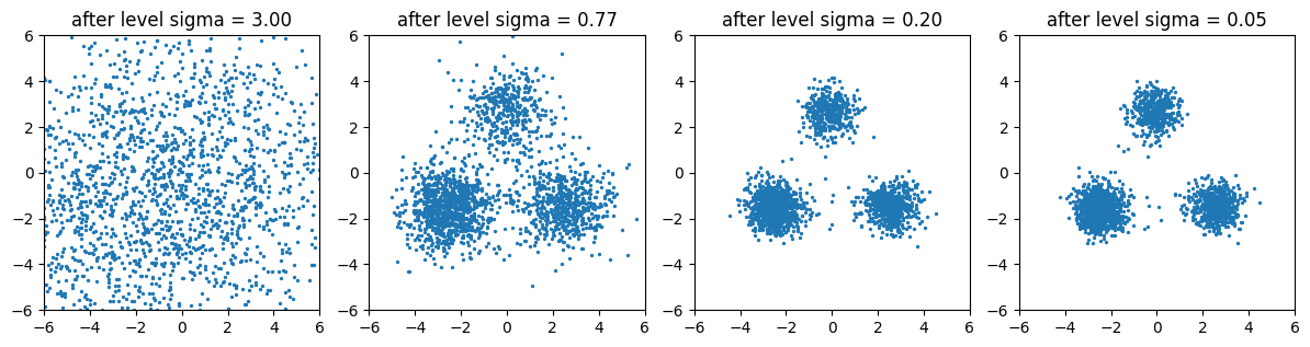
x, snapshots = x_init, []
for i in range(L):
    key, subkey = jax.random.split(key)
    x = annealed_langevin(score, x, subkey, sigmas[i:i + 1])
    if i in (0, 3, 6, 9):
        snapshots.append((float(sigmas[i]), x))
fig, axes = d2l.plt.subplots(1, 4, figsize=(12, 3.3))
for ax, (sigma, pts) in zip(axes, snapshots):
    ax.scatter(pts[:, 0], pts[:, 1], s=2)
    ax.set_xlim(-6, 6), ax.set_ylim(-6, 6), ax.set_aspect('equal')
    ax.set_title(f'after level sigma = {sigma:.2f}')
fig.tight_layout()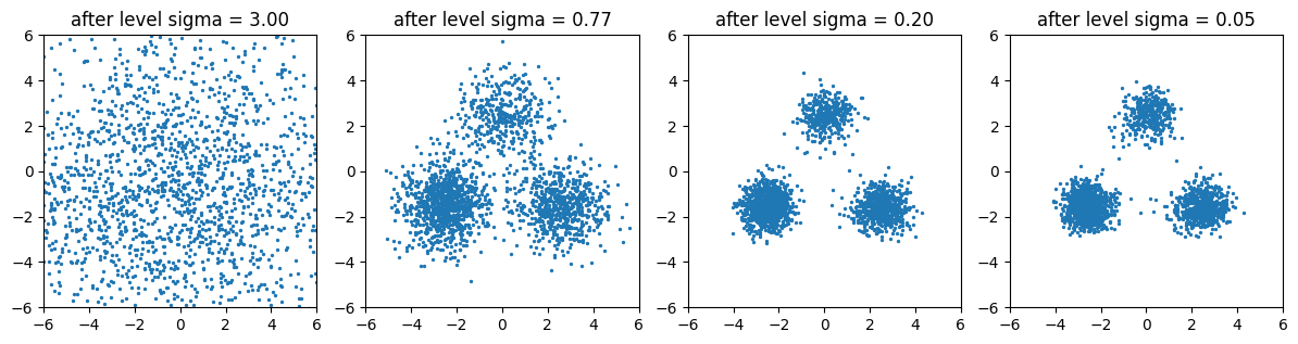
Song and Ermon (2020) describe this coarse-to-fine progression as an iterative refining procedure. For images the same sequence appears as a picture that emerges from noise: typically the coarsest levels fix the global layout and the finer ones add detail, so that each level only has to correct what the previous one left unresolved.
17.6.3 A Noise-Conditional Network for Images
17.6.3.1 The U-Net
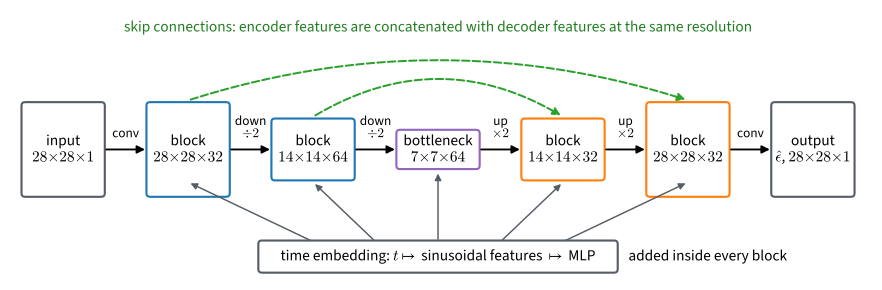
For images the score network must accept a \(28 \times 28\) input, produce an output of the same shape, and take the noise level as a further input. The standard architecture is a U-Net (Ronneberger et al. 2015), adopted in a RefineNet variant for score models by Song and Ermon (2019) and for diffusion models by Ho et al. (2020). An encoder halves the resolution in stages while widening the channels, a decoder reverses the process, and skip connections copy each encoder stage’s features to the decoder stage of the same resolution, so that fine detail does not have to survive the bottleneck (a fully convolutional encoder–decoder without such skip connections serves segmentation in Section 20.11; the U-Net adds them). The noise level enters through an embedding, as in Ho et al. (2020): the level index is mapped to sinusoidal features, as in the positional encodings of Section 10.4, passed through a small multilayer perceptron, and added to the features inside every block (Song and Ermon (2019) instead condition through a modified conditional instance normalization). The class below is a small instance of this design, drawn in Figure 17.6.2, with about 340 thousand parameters. Its cond argument accepts an optional extra embedding, which Section 17.8 uses for class labels, and its channel arguments let Section 17.11 apply the same network to one-hot token images; here both are left at their defaults. The class is saved to the d2l library because the later sections use it unchanged.
def sinusoidal_embedding(t, dim):
    """Map integer steps t (shape (n,)) to sinusoidal features (n, dim)."""
    freqs = torch.exp(-math.log(10000)  # on t's device, so the caller may use a GPU
                      * torch.arange(dim // 2, device=t.device) / (dim // 2))
    args = t.float()[:, None] * freqs[None]
    return torch.cat([torch.sin(args), torch.cos(args)], 1)

class ResBlock(nn.Module):
    """Two 3x3 convolutions with group normalization and an added embedding."""
    def __init__(self, c_in, c_out, emb_dim):
        super().__init__()
        self.norm1 = nn.GroupNorm(8, c_in)
        self.conv1 = nn.Conv2d(c_in, c_out, 3, padding=1)
        self.emb = nn.Linear(emb_dim, c_out)
        self.norm2 = nn.GroupNorm(8, c_out)
        self.conv2 = nn.Conv2d(c_out, c_out, 3, padding=1)
        self.skip = nn.Conv2d(c_in, c_out, 1) if c_in != c_out else nn.Identity()

    def forward(self, x, emb):
        h = self.conv1(nn.functional.silu(self.norm1(x)))
        h = h + self.emb(emb)[:, :, None, None]
        h = self.conv2(nn.functional.silu(self.norm2(h)))
        return h + self.skip(x)

class UNet(nn.Module):
    """A small U-Net for 28x28 images, conditioned on a step index t."""
    def __init__(self, ch=32, emb_dim=128, in_channels=1, out_channels=1):
        super().__init__()
        self.emb_dim = emb_dim
        self.emb_mlp = nn.Sequential(nn.Linear(emb_dim, emb_dim), nn.SiLU(),
                                     nn.Linear(emb_dim, emb_dim))
        self.inc = nn.Conv2d(in_channels, ch, 3, padding=1)
        self.down1 = ResBlock(ch, ch, emb_dim)                    # 28 x 28
        self.pool1 = nn.Conv2d(ch, ch, 3, stride=2, padding=1)    # -> 14 x 14
        self.down2 = ResBlock(ch, 2 * ch, emb_dim)
        self.pool2 = nn.Conv2d(2 * ch, 2 * ch, 3, stride=2, padding=1)  # -> 7 x 7
        self.mid = ResBlock(2 * ch, 2 * ch, emb_dim)
        self.up1 = ResBlock(4 * ch, ch, emb_dim)                  # 14 x 14
        self.up0 = ResBlock(2 * ch, ch, emb_dim)                  # 28 x 28
        self.outc = nn.Sequential(nn.GroupNorm(8, ch), nn.SiLU(),
                                  nn.Conv2d(ch, out_channels, 3, padding=1))

    def forward(self, x, t, cond=None):
        emb = sinusoidal_embedding(t, self.emb_dim)
        if cond is not None:
            emb = emb + cond
        emb = self.emb_mlp(emb)
        h1 = self.down1(self.inc(x), emb)
        h2 = self.down2(self.pool1(h1), emb)
        h = self.mid(self.pool2(h2), emb)
        h = nn.functional.interpolate(h, scale_factor=2, mode='nearest')
        h = self.up1(torch.cat([h, h2], 1), emb)  # skip connection
        h = nn.functional.interpolate(h, scale_factor=2, mode='nearest')
        h = self.up0(torch.cat([h, h1], 1), emb)  # skip connection
        return self.outc(h)
def sinusoidal_embedding(t, dim):
"""Map integer steps t (shape (n,)) to sinusoidal features (n, dim)."""
freqs = jnp.exp(-math.log(10000) * jnp.arange(dim // 2) / (dim // 2))
args = t.astype(jnp.float32)[:, None] * freqs[None]
return jnp.concatenate([jnp.sin(args), jnp.cos(args)], 1)
class ResBlock(nnx.Module):
"""Two 3x3 convolutions with group normalization and an added embedding."""
def __init__(self, c_in, c_out, emb_dim, rngs):
self.norm1 = nnx.GroupNorm(c_in, num_groups=8, rngs=rngs)
self.conv1 = nnx.Conv(c_in, c_out, (3, 3), padding='SAME', rngs=rngs)
self.emb = nnx.Linear(emb_dim, c_out, rngs=rngs)
self.norm2 = nnx.GroupNorm(c_out, num_groups=8, rngs=rngs)
self.conv2 = nnx.Conv(c_out, c_out, (3, 3), padding='SAME', rngs=rngs)
self.skip = (nnx.Conv(c_in, c_out, (1, 1), rngs=rngs) if c_in != c_out
else None)
def __call__(self, x, emb):
h = self.conv1(nnx.silu(self.norm1(x)))
h = h + self.emb(emb)[:, None, None, :]
h = self.conv2(nnx.silu(self.norm2(h)))
return h + (self.skip(x) if self.skip is not None else x)
class UNet(nnx.Module):
"""A small U-Net for 28x28 images (NHWC), conditioned on a step index t."""
def __init__(self, ch=32, emb_dim=128, in_channels=1, out_channels=1,
rngs=None):
self.emb_dim = emb_dim
self.emb1 = nnx.Linear(emb_dim, emb_dim, rngs=rngs)
self.emb2 = nnx.Linear(emb_dim, emb_dim, rngs=rngs)
self.inc = nnx.Conv(in_channels, ch, (3, 3), padding='SAME', rngs=rngs)
self.down1 = ResBlock(ch, ch, emb_dim, rngs) # 28 x 28
self.pool1 = nnx.Conv(ch, ch, (3, 3), strides=2, padding='SAME',
rngs=rngs) # -> 14 x 14
self.down2 = ResBlock(ch, 2 * ch, emb_dim, rngs)
self.pool2 = nnx.Conv(2 * ch, 2 * ch, (3, 3), strides=2,
padding='SAME', rngs=rngs) # -> 7 x 7
self.mid = ResBlock(2 * ch, 2 * ch, emb_dim, rngs)
self.up1 = ResBlock(4 * ch, ch, emb_dim, rngs) # 14 x 14
self.up0 = ResBlock(2 * ch, ch, emb_dim, rngs) # 28 x 28
self.norm = nnx.GroupNorm(ch, num_groups=8, rngs=rngs)
self.outc = nnx.Conv(ch, out_channels, (3, 3), padding='SAME', rngs=rngs)
def __call__(self, x, t, cond=None):
emb = sinusoidal_embedding(t, self.emb_dim)
if cond is not None:
emb = emb + cond
emb = self.emb2(nnx.silu(self.emb1(emb)))
h1 = self.down1(self.inc(x), emb)
h2 = self.down2(self.pool1(h1), emb)
h = self.mid(self.pool2(h2), emb)
h = jnp.repeat(jnp.repeat(h, 2, axis=1), 2, axis=2)
h = self.up1(jnp.concatenate([h, h2], -1), emb) # skip connection
h = jnp.repeat(jnp.repeat(h, 2, axis=1), 2, axis=2)
h = self.up0(jnp.concatenate([h, h1], -1), emb) # skip connection
return self.outc(nnx.silu(self.norm(h)))17.6.3.2 Training and Denoising at Several Levels
We train the U-Net as a noise-conditional score network on Fashion-MNIST, with pixels scaled to \([-1, 1]\) and a ladder of ten levels from \(\sigma_1 = 2\), at which an image is buried in noise, to \(\sigma_L = 0.02\). The network is conditioned on the level index and outputs a noise prediction \(\boldsymbol{\epsilon}_{\boldsymbol{\theta}}\), the convention of Section 17.4 (so that \(\mathbf{f}_{\boldsymbol{\theta}} = -\boldsymbol{\epsilon}_{\boldsymbol{\theta}}\) in the notation above). The loss is Equation 17.6.1 with \(\lambda(\sigma) = \sigma^2\), averaged over pixels, and the score at level \(i\) is \(-\boldsymbol{\epsilon}_{\boldsymbol{\theta}} / \sigma_i\). Six hundred updates take a few minutes on a laptop processor; the published models train for hundreds of thousands.
fmnist = d2l.FashionMNIST(batch_size=128)
X = fmnist.train.data.float()[:, None] / 255 * 2 - 1
X_test = fmnist.val.data.float()[:, None] / 255 * 2 - 1
img_sigmas = torch.exp(torch.linspace(math.log(2.0), math.log(0.02), 10))

torch.manual_seed(4)
unet = UNet()
optimizer = torch.optim.Adam(unet.parameters(), lr=1e-3)
for step in range(600):
    x = X[torch.randint(0, len(X), (128,))]
    level = torch.randint(0, 10, (128,))
    eps = torch.randn_like(x)
    x_noisy = x + img_sigmas[level][:, None, None, None] * eps
    loss = 0.5 * ((unet(x_noisy, level) - eps) ** 2).mean()  # noise prediction
    optimizer.zero_grad(), loss.backward(), optimizer.step()
print(f'final training loss: {loss.item():.3f}')
final training loss: 0.115fmnist = d2l.FashionMNIST(batch_size=128)
X = jnp.asarray(fmnist.train[0], jnp.float32)[..., None] / 255 * 2 - 1
X_test = jnp.asarray(fmnist.val[0], jnp.float32)[..., None] / 255 * 2 - 1
img_sigmas = jnp.exp(jnp.linspace(math.log(2.0), math.log(0.02), 10))
unet = UNet(rngs=nnx.Rngs(4))
optimizer = nnx.Optimizer(unet, optax.adam(1e-3), wrt=nnx.Param)
@nnx.jit
def unet_step(unet, optimizer, x, level, eps):
def loss_fn(model): # noise prediction
x_noisy = x + img_sigmas[level][:, None, None, None] * eps
return 0.5 * ((model(x_noisy, level) - eps) ** 2).mean()
loss, grads = nnx.value_and_grad(loss_fn)(unet)
optimizer.update(unet, grads)
return loss
for step in range(600):
key, k1, k2, k3 = jax.random.split(key, 4)
x = X[jax.random.randint(k1, (128,), 0, len(X))]
loss = unet_step(unet, optimizer, x, jax.random.randint(k2, (128,), 0, 10),
jax.random.normal(k3, x.shape))
print(f'final training loss: {loss:.3f}')final training loss: 0.110One network now approximates the scores of Fashion-MNIST at ten noise levels. The cell checks this claim with Tweedie’s formula Equation 17.4.4 at three of the levels: the same network, told the level, denoises test images corrupted at \(\sigma \approx 0.09\), \(0.43\), and \(2\). It reports the per-pixel squared error before and after denoising and shows, for six images, the clean originals and then the noisy input and the reconstruction at each level, from fine to coarse.
torch.manual_seed(5)
x = X_test[:500]
rows = []
for level in (6, 3, 0):  # sigma about 0.09, 0.43, 2
    sigma = img_sigmas[level]
    x_noisy = x + sigma * torch.randn_like(x)
    with torch.no_grad():
        x_hat = x_noisy - sigma * unet(x_noisy, torch.full((len(x),), level))
    print(f'sigma = {sigma:.2f}: per-pixel squared error noisy {((x_noisy - x) ** 2).mean():.3f}, '
          f'denoised {((x_hat - x) ** 2).mean():.3f}')
    rows += [x_noisy[:6], x_hat[:6]]
imgs = torch.cat([x[:6]] + rows).clamp(-1, 1) / 2 + 0.5
d2l.show_images(imgs.permute(0, 2, 3, 1).repeat(1, 1, 1, 3), 7, 6, scale=0.9);
sigma = 0.09: per-pixel squared error noisy 0.009, denoised 0.002
sigma = 0.43: per-pixel squared error noisy 0.186, denoised 0.022
sigma = 2.00: per-pixel squared error noisy 4.004, denoised 0.132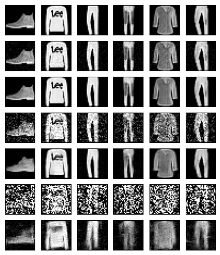
x = X_test[:500]
rows = []
for level in (6, 3, 0):  # sigma about 0.09, 0.43, 2
    sigma = img_sigmas[level]
    key, subkey = jax.random.split(key)
    x_noisy = x + sigma * jax.random.normal(subkey, x.shape)
    x_hat = x_noisy - sigma * unet(x_noisy, jnp.full((len(x),), level))
    print(f'sigma = {sigma:.2f}: per-pixel squared error noisy {((x_noisy - x) ** 2).mean():.3f}, '
          f'denoised {((x_hat - x) ** 2).mean():.3f}')
    rows += [x_noisy[:6], x_hat[:6]]
imgs = jnp.concatenate([x[:6]] + rows).clip(-1, 1) / 2 + 0.5
d2l.show_images(jnp.repeat(imgs, 3, -1), 7, 6, scale=0.9);
sigma = 0.09: per-pixel squared error noisy 0.009, denoised 0.003
sigma = 0.43: per-pixel squared error noisy 0.186, denoised 0.025
sigma = 2.00: per-pixel squared error noisy 4.001, denoised 0.158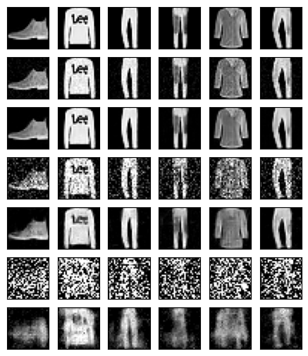
At the fine level the reconstruction is close to the original. At \(\sigma \approx 0.43\) it is the smooth posterior mean seen in Section 17.4. At \(\sigma = 2\) the input is indistinguishable from noise by eye, yet the reconstruction is a blurred silhouette with the original’s overall layout and none of its detail: the posterior mean at such a level averages the many clean images consistent with the noisy input, which share its coarse shape but not its fine structure, and the network has learned what that average looks like. These three reconstructions are the ingredients of iterative refinement: the coarse level supplies the layout, the intermediate level the shape, the fine level the detail. Generating images from scratch with annealed Langevin dynamics requires all ten scores to be accurate, and in particular the intermediate ones on inputs that are not real noisy images but the chain’s own states; Song and Ermon (2019) achieve this with training runs orders of magnitude longer than the one above, and Song and Ermon (2020) refine the choice of ladder, step size, and steps per level. Exercise 6 runs the sampler on this small network. Section 17.8 reaches recognizable samples within the chapter’s budget with the closely related sampler of the next section.
17.6.4 Conditioning through Bayes’ Rule
Score models offer a direct route to conditional generation. Suppose a label \(y\) is attached to each image, and a classifier \(p(y \mid \mathbf{x})\) is available. Bayes’ rule gives \(p(\mathbf{x} \mid y) \propto p(\mathbf{x})\, p(y \mid \mathbf{x})\), and because the score is a gradient in \(\mathbf{x}\), the normalizer \(p(y)\) disappears:
\[ \nabla_{\mathbf{x}} \log p(\mathbf{x} \mid y) = \nabla_{\mathbf{x}} \log p(\mathbf{x}) + \nabla_{\mathbf{x}} \log p(y \mid \mathbf{x}). \tag{17.6.3}\]
The network above learned the unconditional score, and the second term is the input gradient of a classifier. Adding the two and running a score-based sampler, Langevin dynamics here or the diffusion samplers of the later sections, draws from the class-conditional distribution with no retraining of the score network (Song et al. 2021; Dhariwal and Nichol 2021), up to the errors of the learned score, of the classifier, and of the finite chain. Because the sampler operates at each noise level, the classifier must be evaluated on noisy inputs at that level, which requires a classifier trained on noisy data; Section 17.8 trains one and runs this rule as classifier guidance. The same identity underlies the guidance methods used with diffusion models, developed in Section 29.4 and applied in Section 17.8, where the second term is replaced by the difference between a conditional and an unconditional network.
Score-based generative models, as assembled so far, train stably by regression and need no adversary and no normalizer. Their image samples were reported as comparable to those of the adversarial models of the time (Song and Ermon 2019), and, with improved training techniques, as rivaling the best of them on several datasets (Song and Ermon 2020). Three limitations remain. Sampling runs a Markov chain of hundreds or thousands of network evaluations, the model provides no tractable likelihood, and the noise ladder is a sequence of separate distributions rather than a single process with a beginning and an end. The diffusion formulation of the next section addresses the last two, with a single process and a bound on the likelihood; Section 17.9 shortens the chain.
17.6.5 Summary
A noise-conditional score network learns the scores of the Gaussian-perturbed data at a ladder of noise levels with one set of parameters, trained on the denoising objective at every level and weighted by \(\sigma^2\) so that all levels contribute terms of comparable size, which amounts to predicting the added noise. Annealed Langevin dynamics runs the Langevin chain level by level from the coarsest to the finest, with step sizes proportional to \(\sigma_i^2\); each level starts from a sample of the previous one, so the chain is likely to start each level where the current score is well estimated. The mode proportions are settled at the coarse levels, where the chain mixes while the modes are still broad.
On the running example the annealed sampler recovered the mode weights to within a few hundredths, with a slightly inflated spread and about two percent strays, using a thousand network evaluations, whereas the same budget spent at the finest level alone left the weights at their initial values and nearly half of the chains far from every mode. A U-Net conditioned on the level index learned approximations of the scores of Fashion-MNIST at ten noise levels in a few minutes, good enough to denoise at the three levels tested, from the layout at the coarsest to the detail at the finest; generating from noise is left to Exercise 6, and the original work trained for orders of magnitude longer. Bayes’ rule makes conditional sampling a matter of adding a classifier gradient to the score.
17.6.6 Exercises
- The weighting. With the parameterization \(\mathbf{s}_{\boldsymbol{\theta}}(\mathbf{x}, \sigma) = \mathbf{f}_{\boldsymbol{\theta}}(\mathbf{x}, \sigma) / \sigma\), show that the \(\sigma^2\)-weighted denoising objective Equation 17.6.1 equals \(\tfrac{1}{2L} \sum_i \mathbb{E}\|\mathbf{f}_{\boldsymbol{\theta}}(\mathbf{x} + \sigma_i \boldsymbol{\epsilon}, \sigma_i) + \boldsymbol{\epsilon}\|^2\). Then compute, for a single Gaussian data distribution \(\mathcal{N}(0, s^2)\) in one dimension, the value of the unweighted objective at the optimum for each \(\sigma_i\), and explain what an unweighted sum over a ladder from \(\sigma = 3\) to \(\sigma = 0.05\) would emphasize.
- Step sizes. The step size in Equation 17.6.2 is \(\alpha_i = \epsilon\, \sigma_i^2 / \sigma_L^2\). For a single Gaussian target \(p_{\sigma_i} = \mathcal{N}(0, s^2 + \sigma_i^2)\) with \(s \ll \sigma_i\), show that one Langevin step contracts the distance to the mean by the factor \(1 - \alpha_i / (2 (s^2 + \sigma_i^2)) \approx 1 - \epsilon / (2 \sigma_L^2)\), independent of the level. What does this say about the number of steps a level needs, and why is the injected noise \(\sqrt{\alpha_i}\) nevertheless different at every level?
- [code] Exact scores through the ladder. Replace the network in the annealed sampler by the exact score of \(p_{\sigma_i}\), available from
GaussianMixture.scorewith thesigmaargument, and rerun the schedule with \(20\) and \(100\) steps per level, and the thousand-step run at the finest level alone. Compare with the learned-score results and decide which part of each discrepancy from the target is due to the finite chain and which to the learned scores. - [code] The coarsest level. Rerun the annealed sampler with the ladder truncated to start at the level nearest \(0.5\) instead of \(3\), keeping all other settings. Report the mode weights and explain the result using
- [code] A classifier gradient. Label each training point of the running example by the component that generated it, train a small classifier on the noisy points at each level, and add its input gradient to the learned score as in Equation 17.6.3 during annealed sampling. Verify that conditioning on each class produces samples from the corresponding component, and measure the fraction that lands in the wrong one.
- [code] Annealed Langevin on images. Run annealed Langevin dynamics with the trained U-Net, starting from uniform noise on \([-1, 1]\), with \(100\) steps per level and the step-size ratio \(\epsilon / \sigma_L^2 = 0.2\) of Song and Ermon (2019), whose \(\epsilon = 2 \times 10^{-5}\) and \(\sigma_L = 0.01\) refer to pixels in \([0, 1]\) (pass
scale=0.2and the ladderimg_sigmas). The sampler calls its score with noise levels, whereas the U-Net takes a level index and predicts the noise, so wrap it as the score-unet(x, level) / sigma, withlevelthe index of the current level. Display the states after each level. Describe what the coarse levels establish and what the fine levels fail to add at this training budget. Then train for \(3000\) steps instead of \(600\) and repeat.