%matplotlib inline
from d2l import torch as d2l
import math
import torch
from torch import nn17.7 Denoising Diffusion Probabilistic Models
The ladder of the previous section is a collection of separate perturbed distributions, and the sampler that walks down it has a step size and a number of steps per level that must be set by hand. A diffusion model replaces the ladder by a single Markov process that turns data into noise in \(T\) small steps, and it learns the reversal of that process as a latent-variable model, whose training objective derives from a variational bound on the likelihood in the manner of Section 27.3.5. The construction is due to Sohl-Dickstein et al. (2015); Ho et al. (2020) showed that each term of the bound becomes a weighted noise-prediction regression, the same regression as denoising score matching, and that the resulting samples rival those of adversarial models. This section derives the forward process, the bound, the simplification, and the sampler, and checks the marginal, the noise predictor, and the sampler on the running example. The presentation follows lecture 13 of Kuleshov (2023); the monograph of Lai et al. (2025) develops the same derivation and its alternatives at greater length.
%matplotlib inline
from d2l import jax as d2l
import math
import jax
from jax import numpy as jnp
from flax import nnx
import optax
17.7.1 The Forward Process
Fix a number of steps \(T\) and a variance schedule \(\beta_1, \ldots, \beta_T \in (0, 1)\). The forward process starts from a data point \(\mathbf{x}_0 \sim q(\mathbf{x}_0)\), the data distribution (\(q\) denotes every distribution of the forward process), and applies \(T\) Gaussian transitions,
\[ q(\mathbf{x}_t \mid \mathbf{x}_{t-1}) = \mathcal{N}\big(\mathbf{x}_t;\ \sqrt{1 - \beta_t}\, \mathbf{x}_{t-1},\ \beta_t I\big), \qquad q(\mathbf{x}_{1:T} \mid \mathbf{x}_0) = \prod_{t=1}^{T} q(\mathbf{x}_t \mid \mathbf{x}_{t-1}), \tag{17.7.1}\]
each of which shrinks the current state by \(\sqrt{1 - \beta_t}\) and adds noise of variance \(\beta_t\). Ho et al. (2020) use \(T = 1000\) with \(\beta_t\) increasing linearly from \(10^{-4}\) to \(0.02\); the two-dimensional experiments below use \(T = 200\) with a correspondingly larger range. The process is fixed in advance and has no parameters. Figure 17.7.1 shows it as the upper row of arrows.
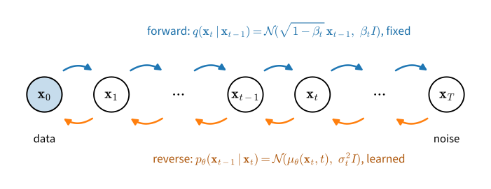
The shrinking factor distinguishes the process from the noise ladder of Section 17.6, which added noise without shrinking. If \(\mathbf{x}_{t-1}\) has identity covariance, then \(\mathbf{x}_t\) has covariance \((1 - \beta_t) I + \beta_t I = I\): the transition preserves unit variance, so the chain moves data toward a standard Gaussian rather than toward an ever wider one, and the end point does not depend on the scale of the data once the remaining signal \(\sqrt{\bar{\alpha}_T}\, \mathbf{x}_0\), defined below, is negligible. Writing \(\alpha_t = 1 - \beta_t\) (the symbol \(\alpha\) is reused here; the Langevin step size of the previous sections is not needed again), a step is \(\mathbf{x}_t = \sqrt{\alpha_t}\, \mathbf{x}_{t-1} + \sqrt{\beta_t}\, \boldsymbol{\epsilon}_t\) with independent \(\boldsymbol{\epsilon}_t \sim \mathcal{N}(\mathbf{0}, I)\).
17.7.1.1 The Marginal in Closed Form
Composing two steps gives \(\mathbf{x}_t = \sqrt{\alpha_t \alpha_{t-1}}\, \mathbf{x}_{t-2} + \sqrt{\alpha_t \beta_{t-1}}\, \boldsymbol{\epsilon}_{t-1} + \sqrt{\beta_t}\, \boldsymbol{\epsilon}_t\). The two noise terms are independent Gaussians, so their sum is a Gaussian with variance \(\alpha_t \beta_{t-1} + \beta_t = \alpha_t (1 - \alpha_{t-1}) + 1 - \alpha_t = 1 - \alpha_t \alpha_{t-1}\). Repeating the argument down to \(\mathbf{x}_0\), with \(\bar{\alpha}_t = \prod_{s=1}^{t} \alpha_s\), gives the marginal of any step directly from the data:
\[ q(\mathbf{x}_t \mid \mathbf{x}_0) = \mathcal{N}\big(\mathbf{x}_t;\ \sqrt{\bar{\alpha}_t}\, \mathbf{x}_0,\ (1 - \bar{\alpha}_t) I\big), \qquad\textrm{i.e.}\qquad \mathbf{x}_t = \sqrt{\bar{\alpha}_t}\, \mathbf{x}_0 + \sqrt{1 - \bar{\alpha}_t}\, \boldsymbol{\epsilon}, \quad \boldsymbol{\epsilon} \sim \mathcal{N}(\mathbf{0}, I). \tag{17.7.2}\]
The formal induction is given in Section 29.4.2.2 (Equation 29.4.8). The formula has two consequences. First, training never needs to simulate the chain: any \(\mathbf{x}_t\) is one Gaussian draw away from \(\mathbf{x}_0\). Second, the marginals are, up to the rescaling by \(\sqrt{\bar{\alpha}_t}\), the noise ladder of Section 17.6. Dividing by \(\sqrt{\bar{\alpha}_t}\) gives \(\mathbf{x}_t / \sqrt{\bar{\alpha}_t} = \mathbf{x}_0 + \sqrt{(1 - \bar{\alpha}_t) / \bar{\alpha}_t}\; \boldsymbol{\epsilon}\), a perturbed copy of the data at a noise level that grows with \(t\). With the schedule of Ho et al. (2020), \(\bar{\alpha}_T \approx 4 \times 10^{-5}\), so \(q(\mathbf{x}_T \mid \mathbf{x}_0)\) is a standard Gaussian to within a scaled-down trace of \(\mathbf{x}_0\), whatever \(\mathbf{x}_0\) was.
The cell sets up the schedule for the running example and checks Equation 17.7.2 by simulation: it runs the chain on the training set and compares the mean and variance of the resulting \(\mathbf{x}_t\) with those of a one-shot draw from the closed form. In the code, index t runs from \(0\) to \(T - 1\) and stands for step \(t + 1\) of the text.
torch.manual_seed(0)
mix = d2l.GaussianMixture(means=[[-2.5, -1.5], [2.5, -1.5], [0.0, 2.5]],
                          weights=[0.5, 0.3, 0.2], std=0.5)
data, test = mix.sample(2000), mix.sample(2000)

T = 200
beta = torch.linspace(1e-4, 0.1, T)
alpha = 1 - beta
alpha_bar = torch.cumprod(alpha, 0)
print(f'alpha_bar_T = {alpha_bar[-1]:.1e}: after T steps the data are scaled '
      f'by {alpha_bar[-1].sqrt():.3f}')

torch.manual_seed(1)
x = data.clone()
for t in range(T):  # the chain, step by step
    x = alpha[t].sqrt() * x + beta[t].sqrt() * torch.randn_like(x)
    if t + 1 in (10, 50, 200):
        one_shot = (alpha_bar[t].sqrt() * data
                    + (1 - alpha_bar[t]).sqrt() * torch.randn_like(data))
        print(f'step {t + 1:3d}: chain: mean {[round(m, 3) for m in x.mean(0).tolist()]}, '
              f'var {x.var(0).mean():.3f} | one shot: mean '
              f'{[round(m, 3) for m in one_shot.mean(0).tolist()]}, '
              f'var {one_shot.var(0).mean():.3f}')
alpha_bar_T = 3.2e-05: after T steps the data are scaled by 0.006
step 10: chain: mean [-0.454, -0.76], var 3.838 | one shot: mean [-0.457, -0.766], var 3.838
step 50: chain: mean [-0.338, -0.563], var 2.554 | one shot: mean [-0.344, -0.553], var 2.554
step 200: chain: mean [-0.036, -0.021], var 0.990 | one shot: mean [-0.003, 0.001], var 0.966key = jax.random.PRNGKey(0)
mix = d2l.GaussianMixture(means=[[-2.5, -1.5], [2.5, -1.5], [0.0, 2.5]],
weights=[0.5, 0.3, 0.2], std=0.5)
key, k1, k2 = jax.random.split(key, 3)
data, test = mix.sample(k1, 2000), mix.sample(k2, 2000)
T = 200
beta = jnp.linspace(1e-4, 0.1, T)
alpha = 1 - beta
alpha_bar = jnp.cumprod(alpha)
print(f'alpha_bar_T = {alpha_bar[-1]:.1e}: after T steps the data are scaled '
f'by {jnp.sqrt(alpha_bar[-1]):.3f}')
x = data
for t in range(T): # the chain, step by step
key, subkey = jax.random.split(key)
x = jnp.sqrt(alpha[t]) * x + jnp.sqrt(beta[t]) * jax.random.normal(subkey, x.shape)
if t + 1 in (10, 50, 200):
key, subkey = jax.random.split(key)
one_shot = (jnp.sqrt(alpha_bar[t]) * data
+ jnp.sqrt(1 - alpha_bar[t]) * jax.random.normal(subkey, data.shape))
print(f'step {t + 1:3d}: chain: mean {[round(float(m), 3) for m in x.mean(0)]}, '
f'var {x.var(0).mean():.3f} | one shot: mean '
f'{[round(float(m), 3) for m in one_shot.mean(0)]}, '
f'var {one_shot.var(0).mean():.3f}')alpha_bar_T = 3.2e-05: after T steps the data are scaled by 0.006
step 10: chain: mean [-0.546, -0.751], var 3.761 | one shot: mean [-0.549, -0.758], var 3.775
step 50: chain: mean [-0.409, -0.601], var 2.489 | one shot: mean [-0.396, -0.531], var 2.500
step 200: chain: mean [-0.005, -0.014], var 1.000 | one shot: mean [-0.001, -0.029], var 0.994The chain and the one-shot draw agree closely at every checkpoint, and after two hundred steps both have mean near zero and unit variance: the mixture has been carried very nearly to a standard Gaussian.
17.7.2 The Reverse Process
Generation runs the chain backward: draw \(\mathbf{x}_T \sim \mathcal{N}(\mathbf{0}, I)\) and sample \(\mathbf{x}_{t-1}\) from the reversal of each forward step until \(\mathbf{x}_0\) is reached. The exact reversal \(q(\mathbf{x}_{t-1} \mid \mathbf{x}_t)\) is, by Bayes’ rule, proportional to \(q(\mathbf{x}_t \mid \mathbf{x}_{t-1})\, q(\mathbf{x}_{t-1})\), and it involves the marginal \(q(\mathbf{x}_{t-1})\), which depends on the entire data distribution and is unavailable. Two facts make it learnable. When the steps are small, the reversal of a Gaussian transition is itself close to a Gaussian, a classical observation that Sohl-Dickstein et al. (2015) turned into a model; in the continuous-time limit the time reversal of the forward diffusion is exactly a diffusion whose drift involves the score of the marginals (Section 29.3.5, (Anderson 1982)). The reverse process is therefore modeled as a Markov chain of Gaussians running from \(T\) to \(0\),
\[ p_{\boldsymbol{\theta}}(\mathbf{x}_{0:T}) = p(\mathbf{x}_T) \prod_{t=1}^{T} p_{\boldsymbol{\theta}}(\mathbf{x}_{t-1} \mid \mathbf{x}_t), \qquad p_{\boldsymbol{\theta}}(\mathbf{x}_{t-1} \mid \mathbf{x}_t) = \mathcal{N}\big(\mathbf{x}_{t-1};\ \boldsymbol{\mu}_{\boldsymbol{\theta}}(\mathbf{x}_t, t),\ \sigma_t^2 I\big), \tag{17.7.3}\]
with \(p(\mathbf{x}_T) = \mathcal{N}(\mathbf{0}, I)\), a mean \(\boldsymbol{\mu}_{\boldsymbol{\theta}}\) computed by a network that receives the current state and the step index, and variances \(\sigma_t^2\) that we fix in advance. Here \(\sigma_t\) is the standard deviation of a reverse step, not the perturbation level \(\sigma_i\) of the previous sections; the noise level of \(\mathbf{x}_t\) is \(\sqrt{1 - \bar{\alpha}_t}\). Ho et al. (2020) found that \(\sigma_t^2 = \beta_t\) and the posterior variance derived below give similar results, and Nichol and Dhariwal (2021) later learned the variances. The intermediate states \(\mathbf{x}_1, \ldots, \mathbf{x}_T\) are latent variables, and the model density of a data point is the marginal \(p_{\boldsymbol{\theta}}(\mathbf{x}_0) = \int p_{\boldsymbol{\theta}}(\mathbf{x}_{0:T})\, d\mathbf{x}_{1:T}\), an integral over \(T\) copies of the data space that is intractable.
17.7.3 The Variational Bound
An intractable marginal likelihood with a tractable joint is the situation of Section 27.3.5, and the same device applies: bound the log-likelihood from below with an auxiliary distribution over the latents. Here the auxiliary distribution is the forward process itself, \(q(\mathbf{x}_{1:T} \mid \mathbf{x}_0)\), which is fixed rather than learned. Multiplying and dividing by it inside the integral and applying Jensen’s inequality (Section 26.3.3) to the concave logarithm,
\[ \log p_{\boldsymbol{\theta}}(\mathbf{x}_0) = \log \mathbb{E}_{q(\mathbf{x}_{1:T} \mid \mathbf{x}_0)}\!\left[ \frac{p_{\boldsymbol{\theta}}(\mathbf{x}_{0:T})}{q(\mathbf{x}_{1:T} \mid \mathbf{x}_0)} \right] \;\geq\; \mathbb{E}_{q(\mathbf{x}_{1:T} \mid \mathbf{x}_0)}\!\left[ \log \frac{p_{\boldsymbol{\theta}}(\mathbf{x}_{0:T})}{q(\mathbf{x}_{1:T} \mid \mathbf{x}_0)} \right] =: -L_{\textrm{VLB}}(\mathbf{x}_0). \tag{17.7.4}\]
The gap between the two sides is the Kullback–Leibler divergence \(\mathrm{KL}\big(q(\mathbf{x}_{1:T} \mid \mathbf{x}_0)\, \|\, p_{\boldsymbol{\theta}}(\mathbf{x}_{1:T} \mid \mathbf{x}_0)\big)\), so minimizing \(L_{\textrm{VLB}}\) pushes the model likelihood up and pulls the learned reverse process toward the true reversal of the forward one.
17.7.3.1 Decomposition into Per-Step Terms
Both processes are Markov chains, and substituting their factorizations turns the bound into a sum of one term per step. Writing \(\mathbb{E}_q\) for the expectation over \(q(\mathbf{x}_{1:T} \mid \mathbf{x}_0)\),
\[ \begin{aligned} L_{\textrm{VLB}} &= \mathbb{E}_q\!\left[ -\log p(\mathbf{x}_T) - \sum_{t=1}^{T} \log \frac{p_{\boldsymbol{\theta}}(\mathbf{x}_{t-1} \mid \mathbf{x}_t)}{q(\mathbf{x}_t \mid \mathbf{x}_{t-1})} \right] \\ &= \mathbb{E}_q\!\left[ -\log p(\mathbf{x}_T) - \sum_{t=2}^{T} \log \left( \frac{p_{\boldsymbol{\theta}}(\mathbf{x}_{t-1} \mid \mathbf{x}_t)}{q(\mathbf{x}_{t-1} \mid \mathbf{x}_t, \mathbf{x}_0)} \cdot \frac{q(\mathbf{x}_{t-1} \mid \mathbf{x}_0)}{q(\mathbf{x}_t \mid \mathbf{x}_0)} \right) - \log \frac{p_{\boldsymbol{\theta}}(\mathbf{x}_0 \mid \mathbf{x}_1)}{q(\mathbf{x}_1 \mid \mathbf{x}_0)} \right] \\ &= \mathbb{E}_q\!\left[ \log \frac{q(\mathbf{x}_T \mid \mathbf{x}_0)}{p(\mathbf{x}_T)} + \sum_{t=2}^{T} \log \frac{q(\mathbf{x}_{t-1} \mid \mathbf{x}_t, \mathbf{x}_0)}{p_{\boldsymbol{\theta}}(\mathbf{x}_{t-1} \mid \mathbf{x}_t)} - \log p_{\boldsymbol{\theta}}(\mathbf{x}_0 \mid \mathbf{x}_1) \right]. \end{aligned} \tag{17.7.5}\]
The second line rewrites each forward transition with \(t \geq 2\) through Bayes’ rule conditioned on \(\mathbf{x}_0\), \(q(\mathbf{x}_t \mid \mathbf{x}_{t-1}) = q(\mathbf{x}_t \mid \mathbf{x}_{t-1}, \mathbf{x}_0) = q(\mathbf{x}_{t-1} \mid \mathbf{x}_t, \mathbf{x}_0)\, q(\mathbf{x}_t \mid \mathbf{x}_0) / q(\mathbf{x}_{t-1} \mid \mathbf{x}_0)\), where the first equality is the Markov property. The third line collapses the telescoping product of the ratios \(q(\mathbf{x}_{t-1} \mid \mathbf{x}_0) / q(\mathbf{x}_t \mid \mathbf{x}_0)\) over \(t = 2, \ldots, T\) into \(q(\mathbf{x}_1 \mid \mathbf{x}_0) / q(\mathbf{x}_T \mid \mathbf{x}_0)\), whose numerator cancels the factor \(q(\mathbf{x}_1 \mid \mathbf{x}_0)\) in the \(t = 1\) term. Each logarithmic ratio in the final line is, in expectation, a Kullback–Leibler divergence between two distributions of the same variable, so
\[ L_{\textrm{VLB}} = \underbrace{\mathrm{KL}\big(q(\mathbf{x}_T \mid \mathbf{x}_0)\, \|\, p(\mathbf{x}_T)\big)}_{L_T} + \sum_{t=2}^{T} \underbrace{\mathbb{E}_q\Big[\mathrm{KL}\big(q(\mathbf{x}_{t-1} \mid \mathbf{x}_t, \mathbf{x}_0)\, \|\, p_{\boldsymbol{\theta}}(\mathbf{x}_{t-1} \mid \mathbf{x}_t)\big)\Big]}_{L_{t-1}} + \underbrace{\mathbb{E}_q\big[-\log p_{\boldsymbol{\theta}}(\mathbf{x}_0 \mid \mathbf{x}_1)\big]}_{L_0}. \tag{17.7.6}\]
The three kinds of terms have different roles (Ho et al. 2020). The prior term \(L_T\) compares the end of the forward chain with the standard Gaussian that the reverse chain starts from; it contains no parameters and is close to zero for a schedule that reaches \(\bar{\alpha}_T \approx 0\). The reconstruction term \(L_0\) scores the final denoising step. The denoising terms \(L_{t-1}\) carry the training signal: each asks the learned transition \(p_{\boldsymbol{\theta}}(\mathbf{x}_{t-1} \mid \mathbf{x}_t)\) to match \(q(\mathbf{x}_{t-1} \mid \mathbf{x}_t, \mathbf{x}_0)\), the reversal of step \(t\) given the clean point. Conditioning on \(\mathbf{x}_0\) is what makes the target tractable: unlike \(q(\mathbf{x}_{t-1} \mid \mathbf{x}_t)\), which requires the data marginal, this posterior involves only the two Gaussian kernels of the forward process.
17.7.3.2 The Forward Posterior
By Bayes’ rule, \(q(\mathbf{x}_{t-1} \mid \mathbf{x}_t, \mathbf{x}_0) \propto q(\mathbf{x}_t \mid \mathbf{x}_{t-1})\, q(\mathbf{x}_{t-1} \mid \mathbf{x}_0)\), a product of two Gaussians in \(\mathbf{x}_{t-1}\): the first has mean \(\mathbf{x}_t / \sqrt{\alpha_t}\) and variance \(\beta_t / \alpha_t\) as a function of \(\mathbf{x}_{t-1}\), and the second has mean \(\sqrt{\bar{\alpha}_{t-1}}\, \mathbf{x}_0\) and variance \(1 - \bar{\alpha}_{t-1}\). Precisions of Gaussian factors add and means combine in proportion to precision, so the posterior is Gaussian, \(q(\mathbf{x}_{t-1} \mid \mathbf{x}_t, \mathbf{x}_0) = \mathcal{N}(\tilde{\boldsymbol{\mu}}_t(\mathbf{x}_t, \mathbf{x}_0), \tilde{\beta}_t I)\), with
\[ \frac{1}{\tilde{\beta}_t} = \frac{\alpha_t}{\beta_t} + \frac{1}{1 - \bar{\alpha}_{t-1}} = \frac{1 - \bar{\alpha}_t}{\beta_t (1 - \bar{\alpha}_{t-1})}, \qquad \tilde{\boldsymbol{\mu}}_t = \frac{\sqrt{\bar{\alpha}_{t-1}}\, \beta_t}{1 - \bar{\alpha}_t}\, \mathbf{x}_0 + \frac{\sqrt{\alpha_t}\, (1 - \bar{\alpha}_{t-1})}{1 - \bar{\alpha}_t}\, \mathbf{x}_t, \tag{17.7.7}\]
where the simplification of the precision uses \(\alpha_t (1 - \bar{\alpha}_{t-1}) + \beta_t = 1 - \bar{\alpha}_t\) (Exercise 2 fills in the algebra). The posterior mean is a linear combination of the clean point and the current noisy point, and its variance \(\tilde{\beta}_t = \beta_t (1 - \bar{\alpha}_{t-1}) / (1 - \bar{\alpha}_t)\) is smaller than \(\beta_t\): much smaller at the first steps, where \(\tilde{\beta}_1 = 0\), and nearly equal once \(\bar{\alpha}_{t-1}\) is well below one.
17.7.4 From the Bound to Noise Prediction
With the reverse variances fixed at \(\sigma_t^2\), each denoising term is a Kullback–Leibler divergence between two isotropic Gaussians whose covariances do not depend on \(\boldsymbol{\theta}\), which by Equation 16.1.7 is a scaled squared distance between their means plus a constant (the constant vanishes when \(\sigma_t^2 = \tilde{\beta}_t\)):
\[ L_{t-1} = \mathbb{E}_q\!\left[ \frac{1}{2 \sigma_t^2} \big\| \tilde{\boldsymbol{\mu}}_t(\mathbf{x}_t, \mathbf{x}_0) - \boldsymbol{\mu}_{\boldsymbol{\theta}}(\mathbf{x}_t, t) \big\|^2 \right] + \textrm{const}. \tag{17.7.8}\]
The network could predict \(\tilde{\boldsymbol{\mu}}_t\) directly. Ho et al. (2020) found that a change of variables gives a target that works about as well with the bound and much better with the simplified loss below. Expressing the clean point through the noise that produced \(\mathbf{x}_t\) in Equation 17.7.2, \(\mathbf{x}_0 = (\mathbf{x}_t - \sqrt{1 - \bar{\alpha}_t}\, \boldsymbol{\epsilon}) / \sqrt{\bar{\alpha}_t}\), and substituting into Equation 17.7.7, the coefficients of \(\mathbf{x}_t\) combine into \(1 / \sqrt{\alpha_t}\) and the posterior mean becomes
\[ \tilde{\boldsymbol{\mu}}_t = \frac{1}{\sqrt{\alpha_t}} \left( \mathbf{x}_t - \frac{\beta_t}{\sqrt{1 - \bar{\alpha}_t}}\, \boldsymbol{\epsilon} \right). \tag{17.7.9}\]
Given \(\mathbf{x}_t\) and \(t\), which the network receives as inputs, everything in this expression is known except \(\boldsymbol{\epsilon}\), so the natural parameterization lets the network predict the noise,
\[ \boldsymbol{\mu}_{\boldsymbol{\theta}}(\mathbf{x}_t, t) = \frac{1}{\sqrt{\alpha_t}} \left( \mathbf{x}_t - \frac{\beta_t}{\sqrt{1 - \bar{\alpha}_t}}\, \boldsymbol{\epsilon}_{\boldsymbol{\theta}}(\mathbf{x}_t, t) \right), \tag{17.7.10}\]
and Equation 17.7.8 becomes a regression of \(\boldsymbol{\epsilon}_{\boldsymbol{\theta}}\) onto \(\boldsymbol{\epsilon}\) with a step-dependent weight:
\[ L_{t-1} = \mathbb{E}_{\mathbf{x}_0, \boldsymbol{\epsilon}}\!\left[ \frac{\beta_t^2}{2 \sigma_t^2 \alpha_t (1 - \bar{\alpha}_t)} \big\| \boldsymbol{\epsilon} - \boldsymbol{\epsilon}_{\boldsymbol{\theta}}\big(\sqrt{\bar{\alpha}_t}\, \mathbf{x}_0 + \sqrt{1 - \bar{\alpha}_t}\, \boldsymbol{\epsilon},\ t\big) \big\|^2 \right] + \textrm{const}. \tag{17.7.11}\]
For \(\sigma_t^2 = \beta_t\) and the schedule used in the code below, the weight in front is about one half at the start of the chain, falls roughly like \(1 / t\) to a tenth of that by \(t = 20\), and stays between about \(0.025\) and \(0.06\) over the rest of the chain; \(\sigma_t^2 = \tilde{\beta}_t\) makes the early weights larger still (Exercise 3 traces both). Ho et al. (2020) drop the weight and also drop the separate treatment of \(L_0\), training instead on the simple loss
\[ L_{\textrm{simple}}(\boldsymbol{\theta}) = \mathbb{E}_{t \sim \mathcal{U}\{1, \ldots, T\},\ \mathbf{x}_0,\ \boldsymbol{\epsilon}}\!\left[ \big\| \boldsymbol{\epsilon} - \boldsymbol{\epsilon}_{\boldsymbol{\theta}}\big(\sqrt{\bar{\alpha}_t}\, \mathbf{x}_0 + \sqrt{1 - \bar{\alpha}_t}\, \boldsymbol{\epsilon},\ t\big) \big\|^2 \right], \tag{17.7.12}\]
a reweighting of the bound that emphasizes the noisier steps, where recovering \(\mathbf{x}_0\) from \(\mathbf{x}_t\) is hardest even though predicting \(\boldsymbol{\epsilon}\) is easiest. Ho et al. (2020) found that it gives better samples than the bound itself. The resulting procedures are short.
Training. Repeat until converged: draw a data point \(\mathbf{x}_0\), a step \(t\) uniformly from \(\{1, \ldots, T\}\), and \(\boldsymbol{\epsilon} \sim \mathcal{N}(\mathbf{0}, I)\); form \(\mathbf{x}_t = \sqrt{\bar{\alpha}_t}\, \mathbf{x}_0 + \sqrt{1 - \bar{\alpha}_t}\, \boldsymbol{\epsilon}\); take a gradient step on \(\|\boldsymbol{\epsilon} - \boldsymbol{\epsilon}_{\boldsymbol{\theta}}(\mathbf{x}_t, t)\|^2\).
Sampling. Draw \(\mathbf{x}_T \sim \mathcal{N}(\mathbf{0}, I)\). For \(t = T, \ldots, 1\): compute \(\boldsymbol{\mu}_{\boldsymbol{\theta}}(\mathbf{x}_t, t)\) from Equation 17.7.10, and set \(\mathbf{x}_{t-1} = \boldsymbol{\mu}_{\boldsymbol{\theta}}(\mathbf{x}_t, t) + \sigma_t \mathbf{z}\) with \(\mathbf{z} \sim \mathcal{N}(\mathbf{0}, I)\) for \(t > 1\) and \(\mathbf{z} = \mathbf{0}\) for \(t = 1\). Return \(\mathbf{x}_0\). The code below uses \(\sigma_t^2 = \beta_t\). This procedure, which draws the root of the chain from the prior and then each variable from the learned conditional given its parent, is called ancestral sampling.
17.7.4.1 The Connection to Score Matching
The regression Equation 17.7.12 is denoising score matching. The conditional score of the marginal Equation 17.7.2 is \(\nabla_{\mathbf{x}_t} \log q(\mathbf{x}_t \mid \mathbf{x}_0) = -\boldsymbol{\epsilon} / \sqrt{1 - \bar{\alpha}_t}\), so a noise predictor and a score model at step \(t\) differ by a constant factor,
\[ \mathbf{s}_{\boldsymbol{\theta}}(\mathbf{x}_t, t) = -\frac{\boldsymbol{\epsilon}_{\boldsymbol{\theta}}(\mathbf{x}_t, t)}{\sqrt{1 - \bar{\alpha}_t}}, \tag{17.7.13}\]
and the simple loss equals twice the noise-conditional denoising objective Equation 17.6.1 with weights \(\lambda_t = 1 - \bar{\alpha}_t\), applied to the scaled data \(\sqrt{\bar{\alpha}_t}\, \mathbf{x}_0\) at the noise levels \(\sqrt{1 - \bar{\alpha}_t}\), which play the role of the \(\sigma_i\) of that objective (Section 29.4.2.2 gives the two-line computation; the appendix writes the objective without the factor \(\tfrac12\), so it states equality). By Vincent’s theorem the minimizer of Equation 17.7.12 over an unrestricted function class is the conditional expectation \(\boldsymbol{\epsilon}^\star(\mathbf{x}_t, t) = \mathbb{E}[\boldsymbol{\epsilon} \mid \mathbf{x}_t] = -\sqrt{1 - \bar{\alpha}_t}\, \nabla_{\mathbf{x}_t} \log q(\mathbf{x}_t)\), where \(q(\mathbf{x}_t)\) is the marginal of the forward process at step \(t\). The sampler is a score-based sampler as well. Substituting Equation 17.7.13 into Equation 17.7.10, one reverse step reads
\[ \mathbf{x}_{t-1} = \frac{1}{\sqrt{\alpha_t}} \Big( \mathbf{x}_t + \beta_t\, \mathbf{s}_{\boldsymbol{\theta}}(\mathbf{x}_t, t) \Big) + \sigma_t \mathbf{z}, \tag{17.7.14}\]
a step of length \(\beta_t\) along the score, twice the drift that Langevin dynamics would use with noise variance \(\beta_t\), followed by Gaussian noise, with a rescaling by \(1 / \sqrt{\alpha_t}\) that undoes the forward shrinkage. It resembles the annealed Langevin update of Section 17.6, with a step size and a noise level per step that the forward process dictates rather than the user. To first order in \(\beta_t\), half of the score step together with the noise is a Langevin step that leaves \(q(\mathbf{x}_t)\) unchanged, and the other half together with the rescaling is a step of the probability-flow equation below, which carries \(q(\mathbf{x}_t)\) to \(q(\mathbf{x}_{t-1})\). Song et al. (2021) identify the whole step as a discretization of the time-reversed diffusion, with Langevin steps as an optional corrector. The two lines of work that this chapter has followed, the variational one from Sohl-Dickstein et al. (2015) and the score-based one from Song and Ermon (2019), arrive at the same kind of model and differ in the forward process: the ladder adds noise without shrinking the data, and the chain shrinks the data as it adds noise (Song et al. 2021; Luo 2022).
The continuous-time view makes the identification exact, and it supplies the vocabulary of the literature. Let the number of steps grow with \(\beta_t = \beta(t/T)/T\) for a rate function \(\beta(\cdot)\) on \([0, 1]\), and write \(t\) from now on for the continuous time \(t/T \in [0, 1]\). The forward chain Equation 17.7.1 then becomes the variance-preserving stochastic differential equation
\[ d\mathbf{x} = -\tfrac{1}{2} \beta(t)\, \mathbf{x}\, dt + \sqrt{\beta(t)}\, d\mathbf{w}, \]
with \(\mathbf{w}\) a Brownian motion, whereas the noise ladder of Section 17.6, which adds noise without shrinking, is the variance-exploding equation \(d\mathbf{x} = \sqrt{d\sigma^2(t)/dt}\, d\mathbf{w}\), with \(\sigma(t)\) the ladder’s noise level as a function of time. Reversing time turns a diffusion into another diffusion whose drift contains the score of the marginal (Anderson 1982),
\[ d\mathbf{x} = \big[ -\tfrac{1}{2} \beta(t)\, \mathbf{x} - \beta(t)\, \nabla_{\mathbf{x}} \log q_t(\mathbf{x}) \big]\, dt + \sqrt{\beta(t)}\, d\bar{\mathbf{w}}, \]
run from \(t = 1\) down to \(0\) with \(\bar{\mathbf{w}}\) a Brownian motion in reversed time; the ancestral step Equation 17.7.14 is a discretization of it. The same marginals are also produced by an ordinary differential equation, the probability-flow equation
\[ d\mathbf{x} = \big[ -\tfrac{1}{2} \beta(t)\, \mathbf{x} - \tfrac{1}{2} \beta(t)\, \nabla_{\mathbf{x}} \log q_t(\mathbf{x}) \big]\, dt, \]
which carries half the score term and no noise. Section 17.9 meets a discretization of this equation. Section 29.4.2.2 identifies the chain with the variance-preserving equation, and Section 29.3.5 and Section 29.3.3.3 derive the reverse-time and the probability-flow equations (Song et al. 2021).
17.7.5 Experiments on the Running Example
The network below predicts the noise from the current point and the step. It is the score network of the earlier sections with a learned embedding of the step index added to its first hidden layer; for \(T = 200\) discrete steps an embedding table is the simplest choice, and the sinusoidal features of Section 17.6 serve the same purpose for the image model of the next section. Training implements the procedure above with the simple loss.
class NoisePredictor(nn.Module):
    def __init__(self, hidden=128):
        super().__init__()
        self.embed = nn.Embedding(T, hidden)  # one learned vector per step
        self.inp = nn.Linear(2, hidden)
        self.net = nn.Sequential(nn.SiLU(), nn.Linear(hidden, hidden),
                                 nn.SiLU(), nn.Linear(hidden, 2))

    def forward(self, x, t):
        return self.net(self.inp(x) + self.embed(t))

def train_ddpm(data, steps=4000, lr=1e-3, seed=2):
    torch.manual_seed(seed)
    net = NoisePredictor()
    optimizer = torch.optim.Adam(net.parameters(), lr=lr)
    for step in range(steps):
        x0 = data[torch.randint(0, len(data), (256,))]
        t = torch.randint(0, T, (256,))
        eps = torch.randn_like(x0)
        x_t = (alpha_bar[t].sqrt()[:, None] * x0
               + (1 - alpha_bar[t]).sqrt()[:, None] * eps)
        loss = ((net(x_t, t) - eps) ** 2).sum(1).mean()  # the simple loss
        optimizer.zero_grad(), loss.backward(), optimizer.step()
    return net

net = train_ddpm(data)
class NoisePredictor(nnx.Module):
def __init__(self, hidden=128, rngs=None):
self.embed = nnx.Embed(T, hidden, # one vector per step, with
embedding_init=nnx.initializers.normal(1.0),
rngs=rngs) # PyTorch's unit-variance init
self.inp = nnx.Linear(2, hidden, rngs=rngs)
self.h = nnx.Linear(hidden, hidden, rngs=rngs)
self.out = nnx.Linear(hidden, 2, rngs=rngs)
def __call__(self, x, t):
h = nnx.silu(self.inp(x) + self.embed(t))
return self.out(nnx.silu(self.h(h)))
@nnx.jit
def ddpm_step(net, optimizer, x0, t, eps):
def loss_fn(model): # the simple loss
x_t = (jnp.sqrt(alpha_bar[t])[:, None] * x0
+ jnp.sqrt(1 - alpha_bar[t])[:, None] * eps)
return ((model(x_t, t) - eps) ** 2).sum(1).mean()
loss, grads = nnx.value_and_grad(loss_fn)(net)
optimizer.update(net, grads)
return loss
def train_ddpm(data, key, steps=4000, lr=1e-3, seed=2):
net = NoisePredictor(rngs=nnx.Rngs(seed))
optimizer = nnx.Optimizer(net, optax.adam(lr), wrt=nnx.Param)
for step in range(steps):
key, k1, k2, k3 = jax.random.split(key, 4)
x0 = data[jax.random.randint(k1, (256,), 0, len(data))]
ddpm_step(net, optimizer, x0, jax.random.randint(k2, (256,), 0, T),
jax.random.normal(k3, x0.shape))
return net
key, subkey = jax.random.split(key)
net = train_ddpm(data, subkey)17.7.5.1 The Learned Predictor against the Optimal One
For the running example the optimal noise predictor is available in closed form: the marginal \(q(\mathbf{x}_t)\) is the mixture with its means scaled by \(\sqrt{\bar{\alpha}_t}\), its component variances scaled by \(\bar{\alpha}_t\), and \(1 - \bar{\alpha}_t\) added to each variance, which is what GaussianMixture.score computes with the scale and sigma arguments, and \(\boldsymbol{\epsilon}^\star = -\sqrt{1 - \bar{\alpha}_t}\) times that score. The cell compares the network with \(\boldsymbol{\epsilon}^\star\) at four steps on noisy test points. It also reports the irreducible part of the loss at each step, \(\mathbb{E}\|\boldsymbol{\epsilon} - \boldsymbol{\epsilon}^\star\|^2\), the variance of the noise that cannot be inferred from \(\mathbf{x}_t\), next to the loss the network attains.
def eps_star(x_t, t):  # the optimal noise predictor at step index t
    a = alpha_bar[t]
    return -(1 - a).sqrt() * mix.score(x_t, scale=a.sqrt().item(),
                                       sigma=(1 - a).sqrt().item())

torch.manual_seed(3)
print(f'{"step":>4} {"E||eps_theta - eps*||^2":>24} {"E||eps - eps*||^2":>18} '
      f'{"E||eps - eps_theta||^2":>23}')
with torch.no_grad():
    for t in (9, 49, 99, 199):
        eps = torch.randn_like(test)
        x_t = alpha_bar[t].sqrt() * test + (1 - alpha_bar[t]).sqrt() * eps
        pred, best = net(x_t, torch.full((len(test),), t)), eps_star(x_t, t)
        print(f'{t + 1:>4} {((pred - best) ** 2).sum(1).mean():>24.3f} '
              f'{((eps - best) ** 2).sum(1).mean():>18.3f} '
              f'{((eps - pred) ** 2).sum(1).mean():>23.3f}')
step E||eps_theta - eps*||^2 E||eps - eps*||^2 E||eps - eps_theta||^2
10 0.056 1.880 1.959
50 0.047 0.714 0.749
100 0.011 0.495 0.507
200 0.007 0.000 0.008def eps_star(x_t, t): # the optimal noise predictor at step index t
a = alpha_bar[t]
return -jnp.sqrt(1 - a) * mix.score(x_t, scale=jnp.sqrt(a),
sigma=jnp.sqrt(1 - a))
print(f'{"step":>4} {"E||eps_theta - eps*||^2":>24} {"E||eps - eps*||^2":>18} '
f'{"E||eps - eps_theta||^2":>23}')
for t in (9, 49, 99, 199):
key, subkey = jax.random.split(key)
eps = jax.random.normal(subkey, test.shape)
x_t = jnp.sqrt(alpha_bar[t]) * test + jnp.sqrt(1 - alpha_bar[t]) * eps
pred, best = net(x_t, jnp.full((len(test),), t)), eps_star(x_t, t)
print(f'{t + 1:>4} {((pred - best) ** 2).sum(1).mean():>24.3f} '
f'{((eps - best) ** 2).sum(1).mean():>18.3f} '
f'{((eps - pred) ** 2).sum(1).mean():>23.3f}')step E||eps_theta - eps*||^2 E||eps - eps*||^2 E||eps - eps_theta||^2
10 0.058 1.779 1.838
50 0.049 0.784 0.831
100 0.010 0.480 0.492
200 0.006 0.000 0.007The mean squared difference between the learned and the optimal predictor is at most a few hundredths at each step checked, on a target with unit variance per coordinate. The second and third columns nearly coincide: the loss the network attains exceeds the irreducible part by less than a tenth, and that part is largest at early steps, where the noise is a small part of \(\mathbf{x}_t\) and hard to separate from the data, and falls nearly to zero at the last step, where \(\mathbf{x}_t\) is almost pure noise and the noise is read off directly. Relative to the bound, the simple loss puts more weight on these late steps, where predicting the noise is easiest.
17.7.5.2 Ancestral Sampling
The sampler implements the procedure above. We run it with the learned predictor and, for reference, with \(\boldsymbol{\epsilon}^\star\), and summarize the samples as in the previous sections.
def ancestral_sample(eps_model, n, snapshot_steps=()):
    """The reverse chain from x_T ~ N(0, I) down to x_0."""
    x, snapshots = torch.randn(n, 2), {}
    with torch.no_grad():
        for t in reversed(range(T)):
            if t + 1 in snapshot_steps:
                snapshots[t + 1] = x.clone()
            eps = eps_model(x, torch.full((n,), t))
            mean = (x - beta[t] / (1 - alpha_bar[t]).sqrt() * eps) / alpha[t].sqrt()
            x = mean + (beta[t].sqrt() * torch.randn_like(x) if t > 0 else 0)
    snapshots[0] = x
    return x, snapshots

def summarize(x):
    d2 = ((x[:, None, :] - mix.means[None]) ** 2).sum(-1)
    weights = [round(w, 3) for w in
               (torch.bincount(d2.argmin(1), minlength=3) / len(x)).tolist()]
    nearest = d2.min(1).values
    inside = nearest < (3 * mix.std) ** 2
    return (f'mode weights {weights}, spread {nearest[inside].mean():.2f}, '
            f'stray {1 - inside.float().mean():.3f}')

torch.manual_seed(4)
print(f'target (2000 samples of the mixture): {summarize(data)}')
samples, snapshots = ancestral_sample(net, 2000, snapshot_steps=(200, 100, 50))
print(f'learned predictor: {summarize(samples)}')
exact, _ = ancestral_sample(lambda x, t: eps_star(x, t[0]), 2000)
print(f'optimal predictor: {summarize(exact)}')
target (2000 samples of the mixture): mode weights [0.5, 0.317, 0.183], spread 0.49, stray 0.012
learned predictor: mode weights [0.498, 0.333, 0.169], spread 0.47, stray 0.024
optimal predictor: mode weights [0.496, 0.283, 0.22], spread 0.49, stray 0.011@nnx.jit
def reverse_step(eps_model, x, t, key):
eps = eps_model(x, jnp.full((len(x),), t))
mean = (x - beta[t] / jnp.sqrt(1 - alpha_bar[t]) * eps) / jnp.sqrt(alpha[t])
return mean + jnp.where(t > 0, jnp.sqrt(beta[t]), 0.0) * jax.random.normal(
key, x.shape)
def ancestral_sample(eps_model, n, key, snapshot_steps=()):
"""The reverse chain from x_T ~ N(0, I) down to x_0."""
key, subkey = jax.random.split(key)
x, snapshots = jax.random.normal(subkey, (n, 2)), {}
for t in reversed(range(T)):
if t + 1 in snapshot_steps:
snapshots[t + 1] = x
key, subkey = jax.random.split(key)
x = reverse_step(eps_model, x, t, subkey)
snapshots[0] = x
return x, snapshots
def summarize(x):
d2 = ((x[:, None, :] - mix.means[None]) ** 2).sum(-1)
weights = [round(float(w), 3) for w in
jnp.bincount(d2.argmin(1), length=3) / len(x)]
nearest = d2.min(1)
inside = nearest < (3 * mix.std) ** 2
return (f'mode weights {weights}, spread {nearest[inside].mean():.2f}, '
f'stray {1 - inside.mean():.3f}')
class OptimalPredictor(nnx.Module): # eps* as a jittable module
def __call__(self, x, t):
return eps_star(x, t[0])
key, k1, k2 = jax.random.split(key, 3)
print(f'target (2000 samples of the mixture): {summarize(data)}')
samples, snapshots = ancestral_sample(net, 2000, k1, snapshot_steps=(200, 100, 50))
print(f'learned predictor: {summarize(samples)}')
exact, _ = ancestral_sample(OptimalPredictor(), 2000, k2)
print(f'optimal predictor: {summarize(exact)}')target (2000 samples of the mixture): mode weights [0.517, 0.296, 0.187], spread 0.46, stray 0.011
learned predictor: mode weights [0.554, 0.274, 0.173], spread 0.46, stray 0.022
optimal predictor: mode weights [0.518, 0.286, 0.197], spread 0.49, stray 0.012Two hundred steps from pure noise reproduce the three modes: with the optimal predictor the weights come within about two hundredths of the true ones and the within-mode spread and the stray fraction match those of exact samples to within sampling error, and with the learned predictor the weights come within about five hundredths. The sampler has no parameters of its own: its step sizes and noise levels are those of the forward schedule. The panels below show the state of the chain at four points on the way down, for the mixture and for a second data set, a noisy spiral, whose structure is not a set of blobs. In both cases the chain starts as a Gaussian cloud and stays one through the first half of the schedule, because the signal in \(\mathbf{x}_t\) is still small there. The mixture’s three blobs have formed by \(t = 50\), whereas the spiral is still diffuse there and takes shape only in the last fifty steps, which also sharpen both.
torch.manual_seed(5)
u = torch.sqrt(torch.rand(2000)) * 3 * math.pi + 0.5
spiral = torch.stack([u * torch.cos(u), u * torch.sin(u)], 1) / 3
spiral = spiral + 0.1 * torch.randn(2000, 2)
net_spiral = train_ddpm(spiral, steps=6000)
_, snapshots_spiral = ancestral_sample(net_spiral, 2000,
                                       snapshot_steps=(200, 100, 50))
fig, axes = d2l.plt.subplots(2, 4, figsize=(12, 6))
for row, snaps in zip(axes, (snapshots, snapshots_spiral)):
    for ax, step in zip(row, (200, 100, 50, 0)):
        ax.scatter(snaps[step][:, 0], snaps[step][:, 1], s=2)
        ax.set_xlim(-5, 5), ax.set_ylim(-5, 5), ax.set_aspect('equal')
        ax.set_title(f't = {step}')
fig.tight_layout()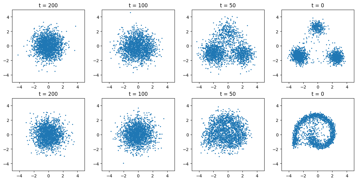
key, k1, k2, k3, k4 = jax.random.split(key, 5)
u = jnp.sqrt(jax.random.uniform(k1, (2000,))) * 3 * math.pi + 0.5
spiral = jnp.stack([u * jnp.cos(u), u * jnp.sin(u)], 1) / 3
spiral = spiral + 0.1 * jax.random.normal(k2, (2000, 2))
net_spiral = train_ddpm(spiral, k3, steps=6000)
_, snapshots_spiral = ancestral_sample(net_spiral, 2000, k4,
                                       snapshot_steps=(200, 100, 50))
fig, axes = d2l.plt.subplots(2, 4, figsize=(12, 6))
for row, snaps in zip(axes, (snapshots, snapshots_spiral)):
    for ax, step in zip(row, (200, 100, 50, 0)):
        ax.scatter(snaps[step][:, 0], snaps[step][:, 1], s=2)
        ax.set_xlim(-5, 5), ax.set_ylim(-5, 5), ax.set_aspect('equal')
        ax.set_title(f't = {step}')
fig.tight_layout()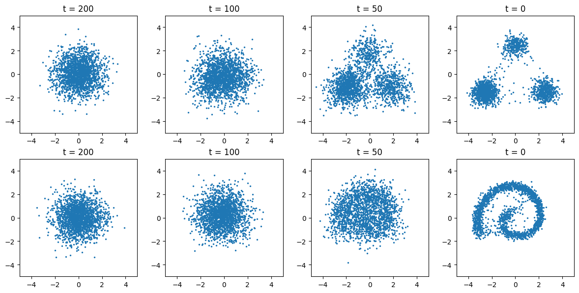
The model of this section trains by a regression with a closed-form target instead of a game, and it rests on a likelihood bound; these answer two of the difficulties that Section 17.1 listed for adversarial training. What it costs is the length of the reverse chain: two hundred network evaluations here, a thousand in the original image models, each a full forward pass. Reducing this cost without retraining is the subject of Section 17.9. The next section scales the model to images.
17.7.6 Summary
A denoising diffusion probabilistic model fixes a forward Markov chain Equation 17.7.1 that shrinks the data and adds Gaussian noise in \(T\) steps, with the closed-form marginal Equation 17.7.2 that lets any step be sampled directly and that ends close to a standard Gaussian. The reverse chain is a latent-variable model with Gaussian transitions whose means a network predicts. The variational bound on the likelihood decomposes into a prior term, a reconstruction term, and one Kullback–Leibler term per step Equation 17.7.6, each comparing the learned transition with the Gaussian posterior \(q(\mathbf{x}_{t-1} \mid \mathbf{x}_t, \mathbf{x}_0)\) of Equation 17.7.7.
Parameterizing the transition mean through a noise prediction turns every step’s term into a weighted regression of the predicted onto the actual noise, and the simple loss Equation 17.7.12 drops the weights. This loss is denoising score matching across the noise levels of the forward process, the optimal predictor is a scaled score of the marginal, and one reverse step resembles a Langevin update with a schedule set by the forward chain and a doubled drift: half of the score step and the noise form a Langevin step at the current level, and the other half with the rescaling carries the chain, to first order, to the next marginal. On the running example, the learned predictor matched the closed-form optimum to within a mean squared error of a few hundredths, its loss exceeded the irreducible noise variance by less than a tenth, and ancestral sampling recovered the mixture with no sampler parameters beyond the forward schedule and the choice \(\sigma_t^2 = \beta_t\).
17.7.7 Exercises
- The marginal by induction. Prove Equation 17.7.2 by induction on \(t\), using that a sum of independent Gaussians is Gaussian with summed variances, and verify the variance-preserving property: if \(\mathbf{x}_0\) has identity covariance, so does every \(\mathbf{x}_t\). Then compute \(\bar{\alpha}_T\) for the schedule of Ho et al. (2020) (\(T = 1000\), \(\beta_t\) linear from \(10^{-4}\) to \(0.02\)), approximating the product by \(\exp(-\sum_t \beta_t)\), and compare with the value of \(\bar{\alpha}_T\) in the code.
- The forward posterior. Multiply the two Gaussian factors of \(q(\mathbf{x}_{t-1} \mid \mathbf{x}_t, \mathbf{x}_0)\), complete the square in \(\mathbf{x}_{t-1}\), and derive Equation 17.7.7. Then substitute \(\mathbf{x}_0 = (\mathbf{x}_t - \sqrt{1 - \bar{\alpha}_t}\, \boldsymbol{\epsilon}) / \sqrt{\bar{\alpha}_t}\) and show that the coefficient of \(\mathbf{x}_t\) in the posterior mean collapses to \(1 / \sqrt{\alpha_t}\), which gives
- [code] The weights of the bound. Compute the weight \(\beta_t^2 / (2 \sigma_t^2 \alpha_t (1 - \bar{\alpha}_t))\) in Equation 17.7.11 for \(\sigma_t^2 = \beta_t\) and for \(\sigma_t^2 = \tilde{\beta}_t\), as a function of \(t = 2, \ldots, T\) for the schedule in the code, and plot both. Which steps does the bound emphasize relative to the simple loss, and how does this relate to the irreducible loss measured in the experiment?
- Two derivations, one model. Starting from Equation 17.7.13, show that the simple loss equals twice the noise-conditional denoising objective Equation 17.6.1 evaluated on the scaled data \(\sqrt{\bar{\alpha}_t}\, \mathbf{x}_0\) at the noise levels of the forward process, with weights \(\lambda_t = 1 - \bar{\alpha}_t\). Then substitute Equation 17.7.13 into Equation 17.7.10 to obtain Equation 17.7.14, and identify the step size and the noise scale of the corresponding Langevin update.
- [code] The prior term. Estimate \(L_T\) for the running example by computing the Kullback–Leibler divergence between \(q(\mathbf{x}_T \mid \mathbf{x}_0)\) and \(\mathcal{N}(\mathbf{0}, I)\) with Equation 16.1.7, averaged over training points. Repeat with \(T = 50\) and the same \(\beta\) range. How large does the prior term become, and what does a large value imply for samples that start from a standard Gaussian?
- [code] Sampling with fewer steps. Run the reverse chain using only every fourth step of the schedule, treating the skipped steps as merged into one transition with the product of their \(\alpha\) values, and compare the summary statistics with the full chain. Then try every tenth step. Where does the approximation break down first: in the mode weights, in the spread, or in the stray fraction?
- [code] Predicting the mean instead of the noise. Train a network to output \(\boldsymbol{\mu}_{\boldsymbol{\theta}}\) directly on the objective Equation 17.7.8 with \(\sigma_t^2 = \beta_t\), using the same architecture and number of updates, and compare the sampling statistics with the noise-prediction model. Explain the difference in the scale of the two regression targets across \(t\).