%matplotlib inline
from d2l import torch as d2l
import math
import torch
from torch import nn17.10 Flow Matching and Its Relation to Diffusion
The chapter has built its generative models from noise: perturb the data, learn the score of the perturbed distribution, and undo the perturbation one level at a time. Section 17.9 ended with the observation that the deterministic version of this procedure integrates an ordinary differential equation. Flow matching (Lipman et al. 2023; Liu et al. 2023; Albergo et al. 2023) starts from that equation. It prescribes a path of distributions from noise to data, learns the velocity field that carries samples along the path, and generates by integrating the field. The construction needs no Markov chain and no variational bound, its training loss has the same form as noise prediction, and it contains diffusion as a special case. For the Gaussian paths used in practice the velocity and the score determine each other by an explicit formula, so a trained noise predictor already defines a velocity field. This formula, a dictionary between the two views, is checked on the running example, where both fields are known in closed form, and the image U-Net is then trained with a velocity target. Section 29.4 proves the two theorems that the section states.
One convention changes. Flow matching runs time in the generative direction: \(t = 0\) is noise and \(t = 1\) is data, the reverse of the diffusion clock, and the paths below are written on this clock.
%matplotlib inline
from d2l import jax as d2l
import jax
from jax import numpy as jnp
from flax import nnx
import optax
17.10.1 Probability Paths and Velocity Fields
A probability path is a family of densities \((p_t)_{t \in [0, 1]}\) with \(p_0 = \mathcal{N}(\mathbf{0}, I)\) and \(p_1 = p_{\textrm{data}}\). A time-dependent velocity field \(\mathbf{u}_t : \mathbb{R}^d \to \mathbb{R}^d\) generates the path if the solution of the ordinary differential equation
\[ \frac{d}{dt} \mathbf{x}_t = \mathbf{u}_t(\mathbf{x}_t), \qquad \mathbf{x}_0 \sim p_0, \tag{17.10.1}\]
has distribution \(p_t\) at every time \(t\). The condition for this is the continuity equation \(\partial_t p_t = -\nabla \cdot (p_t \mathbf{u}_t)\), which states that probability mass moves with the field and is neither created nor destroyed (Section 29.3.3). Given a generating field, sampling is a numerical integration of Equation 17.10.1 from a Gaussian draw to \(t = 1\), with any of the solvers of Section 29.1. The model is a network \(\mathbf{v}_{\boldsymbol{\theta}}(\mathbf{x}, t)\) meant to approximate \(\mathbf{u}_t\), and the natural objective is the flow matching loss \(\mathbb{E}_{t \sim \mathcal{U}[0, 1],\ \mathbf{x} \sim p_t} \|\mathbf{v}_{\boldsymbol{\theta}}(\mathbf{x}, t) - \mathbf{u}_t(\mathbf{x})\|^2\). It has the same defect as explicit score matching: neither \(p_t\) nor \(\mathbf{u}_t\) is available, because both depend on the data distribution, which is known only through samples.
17.10.2 Conditional Flow Matching
The remedy is the one that denoising score matching used. Instead of a path for the whole distribution, prescribe a path for each data point and let the marginal path be their mixture. The simplest choice draws a noise point and a data point independently (the rule for pairing them is called the coupling, and independence is the simplest coupling) and connects them by a straight line traversed at constant speed,
\[ \mathbf{x}_t = (1 - t)\, \mathbf{x}_0 + t\, \mathbf{x}_1, \qquad \mathbf{x}_0 \sim \mathcal{N}(\mathbf{0}, I),\ \mathbf{x}_1 \sim p_{\textrm{data}}, \qquad \frac{d}{dt} \mathbf{x}_t = \mathbf{x}_1 - \mathbf{x}_0 , \tag{17.10.2}\]
the linear path, which Liu et al. (2023) use to define rectified flow. Conditional on the pair, the velocity is the constant \(\mathbf{x}_1 - \mathbf{x}_0\). The marginal \(p_t\) is the distribution of \(\mathbf{x}_t\) when the pair is random: a data point scaled by \(t\) plus Gaussian noise of scale \(1 - t\), which for the running example is again a mixture, with the means scaled by \(t\) and the variance \(t^2 \cdot 0.25 + (1 - t)^2\) per coordinate. Its generating field is the average of the conditional velocities of all the segments passing through a point,
\[ \mathbf{u}_t(\mathbf{x}) = \mathbb{E}\big[ \mathbf{x}_1 - \mathbf{x}_0 \,\big|\, \mathbf{x}_t = \mathbf{x} \big], \tag{17.10.3}\]
a posterior mean of a per-sample quantity, just as the score of the perturbed distribution was the posterior mean of the conditional score in Equation 17.4.3. Two facts make this usable (Lipman et al. 2023). First, the averaged field generates the averaged path: Equation 17.10.3 satisfies the continuity equation for \(p_t\) (the proof differentiates the mixture under the integral sign; see Equation 29.4.14 in the appendix). Second, because a least-squares regression recovers a conditional mean, the conditional flow matching loss
\[ \mathcal{L}_{\textrm{CFM}}(\boldsymbol{\theta}) = \mathbb{E}_{t \sim \mathcal{U}[0, 1],\ \mathbf{x}_0 \sim \mathcal{N}(\mathbf{0}, I),\ \mathbf{x}_1 \sim p_{\textrm{data}}} \left[\, \big\| \mathbf{v}_{\boldsymbol{\theta}}\big( (1 - t)\, \mathbf{x}_0 + t\, \mathbf{x}_1,\ t \big) - (\mathbf{x}_1 - \mathbf{x}_0) \big\|^2 \right] \tag{17.10.4}\]
has the same gradients and the same minimizer as the flow matching loss; the two differ by the expected conditional variance of the target, a constant. The argument is the regression lemma Equation 29.4.5 once more, and Section 29.4.3 gives it in full. Training is therefore as simple as it looks: draw noise, draw data, interpolate, and regress the network’s output onto the difference. The loss floor is again positive, because segments through the same point carry different directions.
The conditional paths are straight, but the trajectories of the marginal field Equation 17.10.3 generally are not: where two segments pass through the same point at the same time, the field averages their directions, and the trajectories of the resulting ODE, which for a smooth field cannot meet at the same point at the same time, bend around one another (Figure 29.4.5). The learned flow’s trajectories decide how few integration steps suffice: the local error of an Euler step is set by the trajectory’s acceleration, which vanishes on straight paths traversed at constant speed; reflow (Liu et al. 2023) retrains on pairs \((\mathbf{x}_0, \mathbf{x}_1)\) that the current model’s own ODE connects, which reduces crossings and straightens the marginal flow, and repeating it straightens the flow further. The experiments below measure how much the trajectories bend, as the excess of their length over the straight-line distance between their ends.
17.10.3 The Relation to Diffusion
Both the linear path and the diffusion process belong to one family. A Gaussian path interpolates between noise and data with time-dependent coefficients,
\[ \mathbf{x}_t = \alpha_t\, \mathbf{x}_1 + \sigma_t\, \boldsymbol{\epsilon}, \qquad \boldsymbol{\epsilon} \sim \mathcal{N}(\mathbf{0}, I), \qquad (\alpha_0, \sigma_0) = (0, 1),\quad (\alpha_1, \sigma_1) = (1, 0), \tag{17.10.5}\]
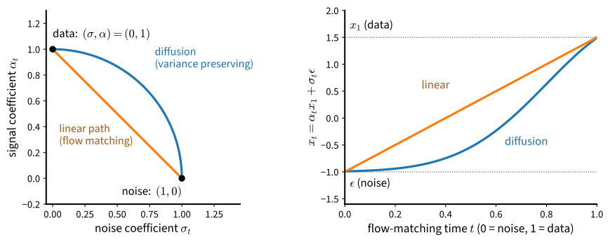
so that \(p_t(\mathbf{x} \mid \mathbf{x}_1) = \mathcal{N}(\alpha_t \mathbf{x}_1, \sigma_t^2 I)\) and the conditional velocity is \(\dot{\alpha}_t \mathbf{x}_1 + \dot{\sigma}_t \boldsymbol{\epsilon}\). Here \(\alpha_t\) and \(\sigma_t\) are the path’s signal and noise coefficients, not the per-step \(\alpha_t = 1 - \beta_t\) or the reverse-step \(\sigma_t\) of the diffusion sections. The linear path is \((\alpha_t, \sigma_t) = (t, 1 - t)\). The diffusion process of Section 17.7, read on the generative clock, is \((\alpha_t, \sigma_t) = (\sqrt{\bar{\alpha}_s}, \sqrt{1 - \bar{\alpha}_s})\) with \(s\) the diffusion step that decreases as \(t\) increases: a variance-preserving path, on which \(\alpha_t^2 + \sigma_t^2 = 1\), and which reaches the noise end only approximately, since \(\bar{\alpha}_T\) is small but not zero. Figure 17.10.1 draws both paths as curves of coefficients and as interpolations of one data value with one noise draw. The two differ in geometry only. The straight path moves at constant speed; the diffusion path keeps \(\alpha_t^2 + \sigma_t^2 = 1\), which preserves the variance of unit-variance data, lingers near the noise end, and accelerates toward the data.
For any Gaussian path the score and the velocity of the marginal are two expressions of the same object.
Proposition (score–velocity dictionary). For the Gaussian path Equation 17.10.5, at every \(t\) with \(\alpha_t, \sigma_t > 0\) and every \(\mathbf{x}\) with \(p_t(\mathbf{x}) > 0\),
\[ \mathbf{u}_t(\mathbf{x}) = \frac{\dot{\alpha}_t}{\alpha_t}\, \mathbf{x} - \left( \sigma_t \dot{\sigma}_t - \sigma_t^2\, \frac{\dot{\alpha}_t}{\alpha_t} \right) \nabla_{\mathbf{x}} \log p_t(\mathbf{x}). \tag{17.10.6}\]
Sketch. Both sides are affine functions of the same posterior mean \(\hat{\mathbf{x}}_1 = \mathbb{E}[\mathbf{x}_1 \mid \mathbf{x}_t = \mathbf{x}]\). The velocity is the posterior mean of \(\dot{\alpha}_t \mathbf{x}_1 + \dot{\sigma}_t \boldsymbol{\epsilon}\) with \(\boldsymbol{\epsilon} = (\mathbf{x} - \alpha_t \mathbf{x}_1) / \sigma_t\), so \(\mathbf{u}_t(\mathbf{x}) = \dot{\alpha}_t \hat{\mathbf{x}}_1 + \dot{\sigma}_t (\mathbf{x} - \alpha_t \hat{\mathbf{x}}_1) / \sigma_t\). The score is the posterior mean of the conditional score \((\alpha_t \mathbf{x}_1 - \mathbf{x}) / \sigma_t^2\) by Vincent’s theorem, so \(\nabla \log p_t(\mathbf{x}) = (\alpha_t \hat{\mathbf{x}}_1 - \mathbf{x}) / \sigma_t^2\), which is Tweedie’s formula Equation 17.4.4 for this kernel. Solving the second relation for \(\hat{\mathbf{x}}_1\) and substituting into the first gives Equation 17.10.6; the full statement is proved in Section 29.4.3.3. \(\blacksquare\)
Three consequences follow. First, a trained diffusion model is a velocity model: the optimal noise prediction is \(\hat{\boldsymbol{\epsilon}} = \mathbb{E}[\boldsymbol{\epsilon} \mid \mathbf{x}_t] = -\sigma_t \nabla \log p_t\) by the same Tweedie computation, so substituting into Equation 17.10.6 gives \(\mathbf{u}_t = (\dot{\alpha}_t / \alpha_t)\, \mathbf{x} + (\dot{\sigma}_t - \sigma_t \dot{\alpha}_t / \alpha_t)\, \hat{\boldsymbol{\epsilon}}\), a velocity computed from the noise predictor of Section 17.7 with no retraining; integrating it is the small-step limit of DDIM, the probability-flow ODE. Second, for the linear path the dictionary reads
\[ \mathbf{u}_t(\mathbf{x}) = \frac{\mathbf{x}}{t} + \frac{1 - t}{t}\, \nabla_{\mathbf{x}} \log p_t(\mathbf{x}), \tag{17.10.7}\]
which for the running example can be evaluated exactly and compared with the learned field. Third, on a given path an ideal network learns the same object whichever of these targets it regresses on, and what distinguishes the two approaches are the choices around it: the path (a straight line against a quarter circle, whose fields differ but, as shown below, are related by a change of time and scale), the regression target (velocity against noise, which differ by a time-dependent affine map and are therefore conditioned differently), and the sampler (an ODE solver against a stochastic chain, a choice that the diffusion side also offers). Kingma and Gao (2023) show that the training objectives of both views are weighted integrals, over noise levels, of the variational bounds of noise-perturbed data; when the weighting is monotonic, as it is for the linear path, the objective equals the variational bound of data augmented with Gaussian noise, so the likelihood interpretation of Section 17.7 carries over in that sense. The learned field also defines a continuous normalizing flow (Section 29.1.5), whose log-density at a sample follows by integrating the field’s divergence along its trajectory (Equation 29.1.10), at the cost of a trace estimate at every solver step; Lipman et al. (2023) present flow matching as a way to train such flows and report likelihoods computed in this way. The linear path with a velocity target is the formulation that Esser et al. (2024) scale to large text-to-image models.
The velocity is also a familiar regression target under another name. On a Gaussian path, the noise \(\boldsymbol{\epsilon}\), the clean point \(\mathbf{x}_1\), and the conditional velocity \(\dot{\alpha}_t \mathbf{x}_1 + \dot{\sigma}_t \boldsymbol{\epsilon}\) are affine functions of one another given \(\mathbf{x}_t\), so a network can be trained to predict any of the three and the others follow; the dictionary of this section is the conversion between them. Predicting \(\mathbf{x}_1\) is \(\mathbf{x}_0\)-prediction in the terminology of diffusion models, and on the variance-preserving path \((\alpha_t, \sigma_t) = (\sin \tfrac{\pi t}{2}, \cos \tfrac{\pi t}{2})\) the conditional velocity equals \(\tfrac{\pi}{2} (\sigma_t \mathbf{x}_1 - \alpha_t \boldsymbol{\epsilon})\), which is, up to the constant factor, the negative of the v-prediction target \(\mathbf{v} = \alpha_t \boldsymbol{\epsilon} - \sigma_t \mathbf{x}_1\) that Salimans and Ho (2022) introduced for stable distillation. The three targets differ in how they weight the noise levels, which Kingma and Gao (2023) make precise.
17.10.4 Experiments on the Running Example
The velocity network is the score network of the earlier sections with the time appended to its input. Training follows Equation 17.10.4 literally.
torch.manual_seed(0)
mix = d2l.GaussianMixture(means=[[-2.5, -1.5], [2.5, -1.5], [0.0, 2.5]],
                          weights=[0.5, 0.3, 0.2], std=0.5)
data, test = mix.sample(2000), mix.sample(2000)

class VelocityNet(nn.Module):
    def __init__(self, hidden=128):
        super().__init__()
        self.net = nn.Sequential(nn.Linear(3, hidden), nn.SiLU(),
                                 nn.Linear(hidden, hidden), nn.SiLU(),
                                 nn.Linear(hidden, 2))

    def forward(self, x, t):
        return self.net(torch.cat([x, t[:, None]], 1))

torch.manual_seed(2)
velocity = VelocityNet()
optimizer = torch.optim.Adam(velocity.parameters(), lr=1e-3)
for step in range(4000):
    x1 = data[torch.randint(0, len(data), (256,))]
    x0, t = torch.randn_like(x1), torch.rand(256)
    x_t = (1 - t)[:, None] * x0 + t[:, None] * x1
    loss = ((velocity(x_t, t) - (x1 - x0)) ** 2).sum(1).mean()
    optimizer.zero_grad(), loss.backward(), optimizer.step()
print(f'final training loss: {loss.item():.3f}')  # dominated by the loss floor
final training loss: 4.499key = jax.random.PRNGKey(0)
mix = d2l.GaussianMixture(means=[[-2.5, -1.5], [2.5, -1.5], [0.0, 2.5]],
weights=[0.5, 0.3, 0.2], std=0.5)
key, k1, k2 = jax.random.split(key, 3)
data, test = mix.sample(k1, 2000), mix.sample(k2, 2000)
class VelocityNet(nnx.Module):
def __init__(self, hidden=128, rngs=None):
self.h1 = nnx.Linear(3, hidden, rngs=rngs)
self.h2 = nnx.Linear(hidden, hidden, rngs=rngs)
self.out = nnx.Linear(hidden, 2, rngs=rngs)
def __call__(self, x, t):
h = jnp.concatenate([x, t[:, None]], 1)
return self.out(nnx.silu(self.h2(nnx.silu(self.h1(h)))))
@nnx.jit
def cfm_step(velocity, optimizer, x0, x1, t):
def loss_fn(model):
x_t = (1 - t)[:, None] * x0 + t[:, None] * x1
return ((model(x_t, t) - (x1 - x0)) ** 2).sum(1).mean()
loss, grads = nnx.value_and_grad(loss_fn)(velocity)
optimizer.update(velocity, grads)
return loss
velocity = VelocityNet(rngs=nnx.Rngs(2))
optimizer = nnx.Optimizer(velocity, optax.adam(1e-3), wrt=nnx.Param)
for step in range(4000):
key, k1, k2, k3 = jax.random.split(key, 4)
x1 = data[jax.random.randint(k1, (256,), 0, len(data))]
loss = cfm_step(velocity, optimizer, jax.random.normal(k2, x1.shape), x1,
jax.random.uniform(k3, (256,)))
print(f'final training loss: {loss:.3f}')final training loss: 4.835The final loss is a few units, far above the values of the earlier sections, because the floor of Equation 17.10.4 is the conditional variance of \(\mathbf{x}_1 - \mathbf{x}_0\) given the interpolated point, which is large near the noise end where the point says little about the data (Exercise 3); the number measures the target’s spread, not the fit.
17.10.4.1 Checking the Dictionary on the Mixture
Equation Equation 17.10.7 expresses the true velocity of the linear path through the score of \(p_t\), which GaussianMixture.score provides with scale = t and sigma = 1 - t. The cell evaluates the learned field and this analytic one on samples from \(p_t\) at four times and reports the mean squared difference next to the mean squared norm of the field.
def true_velocity(x, t):  # the linear-path velocity, from the closed-form score
    return x / t + (1 - t) / t * mix.score(x, scale=t, sigma=1 - t)

print(f'{"t":>4} {"E||v - u||^2":>13} {"E||u||^2":>9}')
with torch.no_grad():
    for t in (0.2, 0.5, 0.8, 0.95):
        x_t = (1 - t) * torch.randn_like(test) + t * test
        u = true_velocity(x_t, t)
        v = velocity(x_t, torch.full((len(test),), t))
        print(f'{t:>4} {((v - u) ** 2).sum(1).mean():>13.3f} {(u ** 2).sum(1).mean():>9.3f}')
t E||v - u||^2 E||u||^2
0.2 0.108 1.079
0.5 0.205 7.803
0.8 0.045 8.052
0.95 0.103 8.352def true_velocity(x, t): # the linear-path velocity, from the closed-form score
return x / t + (1 - t) / t * mix.score(x, scale=t, sigma=1 - t)
print(f'{"t":>4} {"E||v - u||^2":>13} {"E||u||^2":>9}')
for t in (0.2, 0.5, 0.8, 0.95):
key, subkey = jax.random.split(key)
x_t = (1 - t) * jax.random.normal(subkey, test.shape) + t * test
u = true_velocity(x_t, t)
v = velocity(x_t, jnp.full((len(test),), t))
print(f'{t:>4} {((v - u) ** 2).sum(1).mean():>13.3f} {(u ** 2).sum(1).mean():>9.3f}') t E||v - u||^2 E||u||^2
0.2 0.104 1.068
0.5 0.169 7.708
0.8 0.040 8.038
0.95 0.130 8.378The mean squared difference between the learned velocity and the field computed from the score is a few percent of the field’s mean squared norm for \(t \geq 0.5\), a relative error of roughly ten percent in magnitude, and about a tenth of it at \(t = 0.2\), near the noise end, where the field is small and where a regression on the linear path receives its noisiest targets. No score was learned, and no velocity appears in the closed form: the agreement follows from the dictionary.
17.10.4.2 Sampling by Integration
Sampling integrates Equation 17.10.1 with Euler steps. We measure the summary statistics of the previous sections for decreasing numbers of steps, with the learned field and with the exact one, and record the curvature of the trajectories as the excess of the path length over the straight-line distance between start and end, as a fraction of that distance.
@torch.no_grad()
def euler_sample(field, x, steps, record=False):
    trajectory = [x]
    for k in range(steps):
        x = x + field(x, torch.full((len(x),), k / steps)) / steps
        trajectory.append(x)
    return (x, torch.stack(trajectory)) if record else x

def summarize(x):
    d2 = ((x[:, None, :] - mix.means[None]) ** 2).sum(-1)
    weights = [round(w, 3) for w in
               (torch.bincount(d2.argmin(1), minlength=3) / len(x)).tolist()]
    nearest = d2.min(1).values
    inside = nearest < (3 * mix.std) ** 2
    return (f'mode weights {weights}, spread {nearest[inside].mean():.2f}, '
            f'stray {1 - inside.float().mean():.3f}')

def curvature(trajectory):  # path length over chord length, minus one
    length = (trajectory[1:] - trajectory[:-1]).norm(dim=2).sum(0)
    chord = (trajectory[-1] - trajectory[0]).norm(dim=1)
    return (length / chord - 1).mean()

torch.manual_seed(3)
x0 = torch.randn(2000, 2)
print(f'target (2000 samples of the mixture): {summarize(data)}')
for steps in (100, 10, 4, 2):
    print(f'learned field, {steps:>3d} Euler steps: {summarize(euler_sample(velocity, x0, steps))}')
exact = lambda x, t: true_velocity(x, max(t[0].item(), 1e-3))  # avoid t = 0
print(f'exact field,   100 Euler steps: {summarize(euler_sample(exact, x0, 100))}')
_, path = euler_sample(velocity, x0, 100, record=True)
print(f'curvature of the learned flow: {curvature(path):.3f}')
target (2000 samples of the mixture): mode weights [0.5, 0.317, 0.183], spread 0.49, stray 0.012
learned field, 100 Euler steps: mode weights [0.52, 0.322, 0.159], spread 0.50, stray 0.036
learned field, 10 Euler steps: mode weights [0.535, 0.317, 0.148], spread 0.48, stray 0.072
learned field, 4 Euler steps: mode weights [0.596, 0.294, 0.11], spread 0.49, stray 0.175
learned field, 2 Euler steps: mode weights [0.753, 0.214, 0.032], spread 0.76, stray 0.449
exact field, 100 Euler steps: mode weights [0.518, 0.292, 0.19], spread 0.48, stray 0.015
curvature of the learned flow: 0.219def euler_sample(field, x, steps, record=False):
trajectory = [x]
for k in range(steps):
x = x + field(x, jnp.full((len(x),), k / steps)) / steps
trajectory.append(x)
return (x, jnp.stack(trajectory)) if record else x
def summarize(x):
d2 = ((x[:, None, :] - mix.means[None]) ** 2).sum(-1)
weights = [round(float(w), 3) for w in
jnp.bincount(d2.argmin(1), length=3) / len(x)]
nearest = d2.min(1)
inside = nearest < (3 * mix.std) ** 2
return (f'mode weights {weights}, spread {nearest[inside].mean():.2f}, '
f'stray {1 - inside.mean():.3f}')
def curvature(trajectory): # path length over chord length, minus one
length = jnp.linalg.norm(trajectory[1:] - trajectory[:-1], axis=2).sum(0)
chord = jnp.linalg.norm(trajectory[-1] - trajectory[0], axis=1)
return (length / chord - 1).mean()
key, subkey = jax.random.split(key)
x0 = jax.random.normal(subkey, (2000, 2))
print(f'target (2000 samples of the mixture): {summarize(data)}')
for steps in (100, 10, 4, 2):
print(f'learned field, {steps:>3d} Euler steps: {summarize(euler_sample(velocity, x0, steps))}')
exact = lambda x, t: true_velocity(x, jnp.maximum(t[0], 1e-3)) # avoid t = 0
print(f'exact field, 100 Euler steps: {summarize(euler_sample(exact, x0, 100))}')
_, path = euler_sample(velocity, x0, 100, record=True)
print(f'curvature of the learned flow: {curvature(path):.3f}')target (2000 samples of the mixture): mode weights [0.517, 0.296, 0.187], spread 0.46, stray 0.011
learned field, 100 Euler steps: mode weights [0.523, 0.291, 0.187], spread 0.47, stray 0.038
learned field, 10 Euler steps: mode weights [0.543, 0.285, 0.173], spread 0.46, stray 0.068
learned field, 4 Euler steps: mode weights [0.617, 0.26, 0.124], spread 0.51, stray 0.153
learned field, 2 Euler steps: mode weights [0.78, 0.18, 0.041], spread 0.76, stray 0.278
exact field, 100 Euler steps: mode weights [0.521, 0.276, 0.203], spread 0.47, stray 0.010
curvature of the learned flow: 0.200A hundred Euler steps come within a few hundredths of the mixture’s weights, with a few percent of stray points; ten remain close; four and two degrade, with the stray fraction rising first. The curvature explains the trend: the learned flow’s trajectories are longer than their chords by about a fifth, so a handful of straight Euler steps cannot follow them. This curvature belongs to the marginal field, not to the network. The exact field, integrated with a hundred steps, reproduces the target statistics, with about one percent strays as in the data, so the learned field’s extra strays are learning error. (The code evaluates the exact field at \(t = 10^{-3}\) in place of \(t = 0\), because the dictionary divides by \(t\), although the field itself has a finite limit there.) The next cell shows that the exact trajectories, from the same two thousand starting points, are curved to the same degree as the learned ones. To see the geometry without the learning error, the panels integrate eight starting points along the exact field of the linear path and along the exact velocity of a variance-preserving path, the cosine schedule \((\alpha_t, \sigma_t) = (\sin \tfrac{\pi t}{2}, \cos \tfrac{\pi t}{2})\) (a smooth stand-in for the DDPM schedule, which is also variance preserving), obtained from the dictionary Equation 17.10.6 with the closed-form score. Both fields carry the same Gaussian to the same mixture; they differ in the scale and the pace of the route.
def vp_velocity(x, t):  # the dictionary on the cosine variance-preserving path
    t = max(t[0].item(), 1e-3)  # the dictionary divides by alpha_t, zero at t = 0
    alpha, sigma = math.sin(math.pi * t / 2), math.cos(math.pi * t / 2)
    dalpha, dsigma = math.pi / 2 * sigma, -math.pi / 2 * alpha  # time derivatives
    score = mix.score(x, scale=alpha, sigma=sigma)
    return dalpha / alpha * x - (sigma * dsigma - sigma ** 2 * dalpha / alpha) * score

torch.manual_seed(4)
starts, paths = torch.randn(8, 2), {}
for title, field in (('linear path', exact), ('variance-preserving path', vp_velocity)):
    _, path = euler_sample(field, x0, 100, record=True)  # the 2000 starts of above
    print(f'curvature of the exact flow, {title}: {curvature(path):.3f}')
    _, paths[title] = euler_sample(field, starts, 100, record=True)  # for drawing
axis = torch.linspace(-6, 6, 121)
grid = torch.stack(torch.meshgrid(axis, axis, indexing='ij'), -1).reshape(-1, 2)
density = torch.exp(mix.log_prob(grid)).reshape(121, 121).T
fig, axes = d2l.plt.subplots(1, 2, figsize=(8.5, 4.2))
for ax, (title, path) in zip(axes, paths.items()):
    ax.contourf(axis, axis, density, levels=12, cmap='Blues')
    for i in range(8):
        ax.plot(path[:, i, 0], path[:, i, 1], lw=0.9)
        ax.plot(path[0, i, 0], path[0, i, 1], 'ko', ms=3)
    ax.set_title(title), ax.set_aspect('equal')
fig.tight_layout()
curvature of the exact flow, linear path: 0.213
curvature of the exact flow, variance-preserving path: 0.105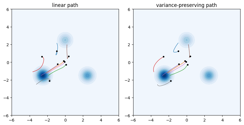
def vp_velocity(x, t):  # the dictionary on the cosine variance-preserving path
    t = jnp.maximum(t[0], 1e-3)  # the dictionary divides by alpha_t, zero at t = 0
    alpha, sigma = jnp.sin(jnp.pi * t / 2), jnp.cos(jnp.pi * t / 2)
    dalpha, dsigma = jnp.pi / 2 * sigma, -jnp.pi / 2 * alpha  # time derivatives
    score = mix.score(x, scale=alpha, sigma=sigma)
    return dalpha / alpha * x - (sigma * dsigma - sigma ** 2 * dalpha / alpha) * score

key, subkey = jax.random.split(key)
starts, paths = jax.random.normal(subkey, (8, 2)), {}
for title, field in (('linear path', exact), ('variance-preserving path', vp_velocity)):
    _, path = euler_sample(field, x0, 100, record=True)  # the 2000 starts of above
    print(f'curvature of the exact flow, {title}: {curvature(path):.3f}')
    _, paths[title] = euler_sample(field, starts, 100, record=True)  # for drawing
axis = jnp.linspace(-6, 6, 121)
grid = jnp.stack(jnp.meshgrid(axis, axis, indexing='ij'), -1).reshape(-1, 2)
density = jnp.exp(mix.log_prob(grid)).reshape(121, 121).T
fig, axes = d2l.plt.subplots(1, 2, figsize=(8.5, 4.2))
for ax, (title, path) in zip(axes, paths.items()):
    ax.contourf(axis, axis, density, levels=12, cmap='Blues')
    for i in range(8):
        ax.plot(path[:, i, 0], path[:, i, 1], lw=0.9)
        ax.plot(path[0, i, 0], path[0, i, 1], 'ko', ms=3)
    ax.set_title(title), ax.set_aspect('equal')
fig.tight_layout()
curvature of the exact flow, linear path: 0.213
curvature of the exact flow, variance-preserving path: 0.105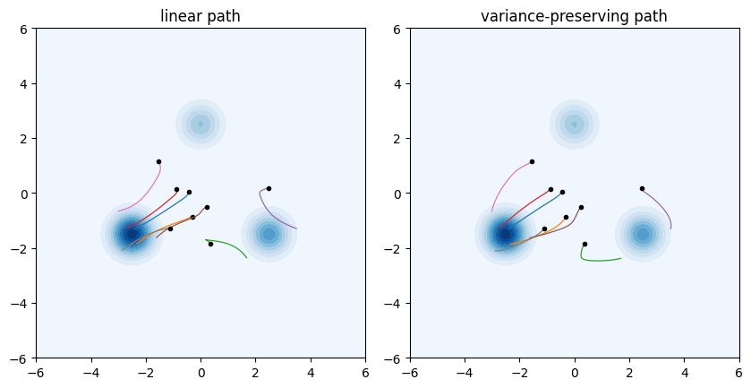
Neither route is straight, and the dictionary relates the two exactly. After reparameterizing time so that the two paths have the same ratio \(\alpha_t / \sigma_t\), and hence the same signal-to-noise ratio \(\alpha_t^2 / \sigma_t^2\), at every instant, their marginals differ only by a scale factor, and substituting into Equation 17.10.6 shows that their velocity fields then map onto each other under that scaling (Exercise 4). The trajectories of two Gaussian paths therefore differ only by a time-dependent rescaling and by the pace at which they are traversed (Karras et al. 2022). The rescaling changes the curvature, and on this example it makes the variance-preserving route about half as curved as the linear one. The straightness of the conditional segments does not transfer to the marginal flow, so a straight conditional path does not by itself give few-step sampling. What does is a straight marginal flow traversed at constant speed, which reflow approaches by changing the coupling between noise and data rather than the path; the distillation methods mentioned in Section 17.8 sidestep the curvature instead by learning the multi-step map directly.
17.10.5 Images with a Velocity Target
The image model changes in two lines: the input is the linear interpolation rather than the diffusion marginal, and the target is \(\mathbf{x}_1 - \mathbf{x}_0\) rather than \(\boldsymbol{\epsilon}\). The U-Net of Section 17.6 expects an integer-like step index for its embedding, so we pass \(1000 t\). Training runs for a thousand updates, as for the unconditional model of Section 17.9, with the moving average of Section 17.8, and sampling integrates the field with fifty Euler steps.
fmnist = d2l.FashionMNIST(batch_size=128)
X = fmnist.train.data.float()[:, None] / 255 * 2 - 1

torch.manual_seed(5)
unet = d2l.UNet()
ema = d2l.UNet()
ema.load_state_dict(unet.state_dict())
optimizer = torch.optim.Adam(unet.parameters(), lr=1e-3)
for step in range(1000):
    x1 = X[torch.randint(0, len(X), (128,))]
    x0, t = torch.randn_like(x1), torch.rand(128)
    x_t = (1 - t)[:, None, None, None] * x0 + t[:, None, None, None] * x1
    loss = ((unet(x_t, 1000 * t) - (x1 - x0)) ** 2).mean()
    optimizer.zero_grad(), loss.backward(), optimizer.step()
    decay = min(0.999, (1 + step) / (10 + step))
    with torch.no_grad():
        for p_ema, p in zip(ema.parameters(), unet.parameters()):
            p_ema.mul_(decay).add_(p, alpha=1 - decay)
print(f'final training loss: {loss.item():.3f}')

torch.manual_seed(6)
x = torch.randn(48, 1, 28, 28)
with torch.no_grad():
    for k in range(50):
        x = x + ema(x, torch.full((48,), 1000 * k / 50)) / 50
imgs = x.clamp(-1, 1) / 2 + 0.5
d2l.show_images(imgs.permute(0, 2, 3, 1).repeat(1, 1, 1, 3), 6, 8, scale=0.8);
final training loss: 0.280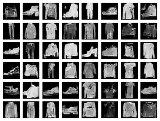
fmnist = d2l.FashionMNIST(batch_size=128)
X = jnp.asarray(fmnist.train[0], jnp.float32)[..., None] / 255 * 2 - 1

unet = d2l.UNet(rngs=nnx.Rngs(5))
graphdef, ema_state = nnx.split(unet)
optimizer = nnx.Optimizer(unet, optax.adam(1e-3), wrt=nnx.Param)

@nnx.jit
def unet_step(unet, optimizer, x0, x1, t):
    def loss_fn(model):
        x_t = (1 - t)[:, None, None, None] * x0 + t[:, None, None, None] * x1
        return ((model(x_t, 1000 * t) - (x1 - x0)) ** 2).mean()
    loss, grads = nnx.value_and_grad(loss_fn)(unet)
    optimizer.update(unet, grads)
    return loss

@jax.jit
def ema_update(ema_state, state, decay):
    return jax.tree_util.tree_map(lambda e, p: decay * e + (1 - decay) * p,
                                  ema_state, state)

for step in range(1000):
    key, k1, k2, k3 = jax.random.split(key, 4)
    x1 = X[jax.random.randint(k1, (128,), 0, len(X))]
    loss = unet_step(unet, optimizer, jax.random.normal(k2, x1.shape), x1,
                     jax.random.uniform(k3, (128,)))
    ema_state = ema_update(ema_state, nnx.state(unet),
                           min(0.999, (1 + step) / (10 + step)))
ema = nnx.merge(graphdef, ema_state)
print(f'final training loss: {loss:.3f}')

@nnx.jit
def euler_image_step(model, x, t, dt):
    return x + model(x, jnp.full((len(x),), 1000 * t)) * dt

key, subkey = jax.random.split(key)
x = jax.random.normal(subkey, (48, 28, 28, 1))
for k in range(50):
    x = euler_image_step(ema, x, k / 50, 1 / 50)
imgs = x.clip(-1, 1) / 2 + 0.5
d2l.show_images(jnp.repeat(imgs, 3, -1), 6, 8, scale=0.8);
final training loss: 0.273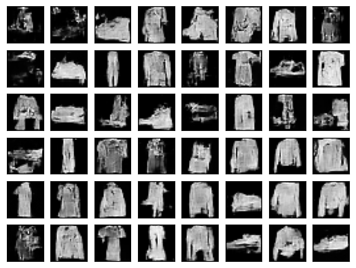
Fifty Euler steps along the learned velocity produce Fashion-MNIST samples of the same character as the DDIM samples of Section 17.9, from the same architecture, the same data, and the same number of updates. The change of path and target left the architecture untouched and replaced the thousand-step chain by a fifty-step integration from the start.
17.10.6 Summary
Flow matching prescribes a path of distributions from a Gaussian to the data and learns the velocity field that generates it; sampling integrates the field. Conditional flow matching makes the objective tractable in the same way as denoising score matching: the marginal velocity is the posterior mean of a conditional velocity, and regressing onto the conditional velocity of a straight noise-to-data segment, Equation 17.10.4, trains the marginal field. On the running example the learned field agreed with the analytic velocity derived from the closed-form score, and a hundred Euler steps came within a few hundredths of the mixture’s weights.
Diffusion is the same construction on a different Gaussian path. The dictionary Equation 17.10.6 converts the score, or the noise prediction, of any Gaussian path into its velocity, so a diffusion model is a flow model whose path is the variance-preserving quarter circle and whose deterministic sampler, DDIM, is an integrator of the resulting ODE. The two views differ in the geometry of the path, in the conditioning and the weighting of the regression target, and in the sampler. On a given path an ideal network learns the same object whichever target it regresses on, and the fields of different Gaussian paths are related by a change of time and scale. The marginal flow is curved under both paths, which is why accurate sampling needs many Euler steps, a higher-order solver, a straightened coupling, or distillation. Every path of this section, like every diffusion model of the chapter so far, adds Gaussian noise to continuous data; the next section drops that assumption.
17.10.7 Exercises
- The marginal of the linear path. For the running example, derive the density \(p_t\) of \(\mathbf{x}_t = (1 - t)\, \mathbf{x}_0 + t\, \mathbf{x}_1\) and confirm that it is the mixture with means \(t \boldsymbol{\mu}_k\) and per-coordinate variance \(t^2 \cdot 0.25 + (1 - t)^2\). Then derive Equation 17.10.7 from Equation 17.10.6 with \((\alpha_t, \sigma_t) = (t, 1 - t)\).
- Noise prediction as a velocity. Substitute \(\nabla \log p_t = -\hat{\boldsymbol{\epsilon}} / \sigma_t\) into Equation 17.10.6 and obtain the velocity in terms of the noise prediction. Specialize to the variance-preserving path \(\alpha_t^2 + \sigma_t^2 = 1\) and show that the coefficient of \(\hat{\boldsymbol{\epsilon}}\) becomes \(\dot{\sigma}_t (\alpha_t^2 + \sigma_t^2) / \alpha_t^2 = \dot{\sigma}_t / \alpha_t^2\) after using \(\alpha_t \dot{\alpha}_t = -\sigma_t \dot{\sigma}_t\).
- The loss floor. Show that the conditional flow matching loss at its minimum equals \(\mathbb{E}_{t, \mathbf{x}_t}\, \mathrm{Var}[\mathbf{x}_1 - \mathbf{x}_0 \mid \mathbf{x}_t]\), with the variance summed over coordinates. For one-dimensional Gaussian data with variance \(s^2\), show that the floor at time \(t\) is \(s^2 / (s^2 t^2 + (1 - t)^2)\), which equals \(s^2\) at the noise end and \(1\) at the data end. At which \(t\) is it largest? Why is the floor large near the noise end for the running example, whose coordinates have variances of about \(5\) and \(2.8\)?
- Same ratio, same flow. Let two Gaussian paths have coefficients related by \(\alpha^B_t = c_t\, \alpha^A_t\) and \(\sigma^B_t = c_t\, \sigma^A_t\) for a positive function \(c_t\), so that they share the signal-to-noise ratio at every time. Show that their marginals satisfy \(p^B_t(\mathbf{y}) = c_t^{-d}\, p^A_t(\mathbf{y} / c_t)\), and use Equation 17.10.6 to show that \(\mathbf{u}^B_t(\mathbf{y}) = (\dot{c}_t / c_t)\, \mathbf{y} + c_t\, \mathbf{u}^A_t(\mathbf{y} / c_t)\). Conclude that the ODE trajectories are related by \(\mathbf{y}_t = c_t\, \mathbf{x}_t\). Which function of the path therefore determines the shape of the route, up to this rescaling?
- [code] Higher-order integration. Replace the Euler step by the midpoint rule (two field evaluations per step) and compare the summary statistics at equal numbers of field evaluations: Euler with \(10\) steps against midpoint with \(5\). Repeat with the exact field to separate the integration error from the learning error.
- [code] Reflow. Generate \(2000\) pairs \((\mathbf{x}_0, \hat{\mathbf{x}}_1)\) by integrating the learned flow from Gaussian draws with a hundred steps, retrain the velocity network on these pairs instead of independent noise-data pairs, and measure the curvature of the new flow and the two-step sampling statistics. Explain why the coupling matters.
- [code] A diffusion model as a flow. Train the noise predictor of Section 17.7 on the mixture, convert it to a velocity with the formula of Exercise 2 on the variance-preserving path of the DDPM schedule, and integrate with Euler on the flow clock. Compare the samples with DDIM at the same number of steps and explain the relation between the two procedures.