%matplotlib inline
from d2l import torch as d2l
import torch
from torch import nn17.9 Denoising Diffusion Implicit Models
Every sample of Section 17.8 took a thousand steps of the reverse chain, each a forward pass of the U-Net, because the chain was built to undo the forward process one small step at a time. The training objective, however, never looked at the chain as a whole. The simple loss Equation 17.7.12 depends only on the marginals \(q(\mathbf{x}_t \mid \mathbf{x}_0)\), and many forward processes share those marginals. Song et al. (2021) exploit this freedom: they construct a family of non-Markovian forward processes with the same marginals as DDPM, derive the corresponding reverse samplers, and show that the family can be sampled on a sparse subset of the steps, its deterministic member best. The result, the denoising diffusion implicit model (DDIM), uses the trained noise predictor without retraining and, for a well-trained predictor, reaches comparable samples in a few dozen evaluations. The derivation below is checked on the running example, where the error of skipping steps can be measured exactly, and then applied to the Fashion-MNIST model.
%matplotlib inline
from d2l import jax as d2l
import jax
from jax import numpy as jnp
from flax import nnx
import optax
17.9.1 Forward Processes with the Same Marginals
Fix the schedule \(\bar{\alpha}_1, \ldots, \bar{\alpha}_T\) of a DDPM and a sequence of nonnegative numbers \(\sigma_1, \ldots, \sigma_T\). Instead of specifying the forward process by its transitions \(q(\mathbf{x}_t \mid \mathbf{x}_{t-1})\), specify it by its terminal marginal and by the conditionals of each step given the clean point:
\[ q_\sigma(\mathbf{x}_{1:T} \mid \mathbf{x}_0) = q_\sigma(\mathbf{x}_T \mid \mathbf{x}_0) \prod_{t=2}^{T} q_\sigma(\mathbf{x}_{t-1} \mid \mathbf{x}_t, \mathbf{x}_0), \qquad q_\sigma(\mathbf{x}_T \mid \mathbf{x}_0) = \mathcal{N}\big(\sqrt{\bar{\alpha}_T}\, \mathbf{x}_0,\ (1 - \bar{\alpha}_T) I\big), \]
\[ q_\sigma(\mathbf{x}_{t-1} \mid \mathbf{x}_t, \mathbf{x}_0) = \mathcal{N}\!\left( \sqrt{\bar{\alpha}_{t-1}}\, \mathbf{x}_0 + \sqrt{1 - \bar{\alpha}_{t-1} - \sigma_t^2}\; \frac{\mathbf{x}_t - \sqrt{\bar{\alpha}_t}\, \mathbf{x}_0}{\sqrt{1 - \bar{\alpha}_t}},\ \sigma_t^2 I \right). \tag{17.9.1}\]
The mean of each conditional is a combination of the clean point and of the direction from the clean point to \(\mathbf{x}_t\), rescaled from noise level \(t\) to noise level \(t - 1\), and \(\sigma_t\) sets how much fresh noise is added on the way. (These \(\sigma_t\) are the noise scales of this family, not the perturbation levels of the earlier sections.) By Bayes’ rule the forward step \(q_\sigma(\mathbf{x}_t \mid \mathbf{x}_{t-1}, \mathbf{x}_0)\) is again Gaussian, but its mean depends on \(\mathbf{x}_0\) as well as on \(\mathbf{x}_{t-1}\), so the process is not Markov in general (Song et al. 2021); the DDPM member below is the exception. What the family shares with DDPM is the marginals.
Proposition. For every choice of \(\sigma\) with \(\sigma_t^2 \leq 1 - \bar{\alpha}_{t-1}\), the marginals of Equation 17.9.1 are those of DDPM: \(q_\sigma(\mathbf{x}_t \mid \mathbf{x}_0) = \mathcal{N}(\sqrt{\bar{\alpha}_t}\, \mathbf{x}_0, (1 - \bar{\alpha}_t) I)\) for all \(t\).
Proof. By backward induction on \(t\). The claim holds at \(t = T\) by construction. If it holds at \(t\), write \(\mathbf{x}_t = \sqrt{\bar{\alpha}_t}\, \mathbf{x}_0 + \sqrt{1 - \bar{\alpha}_t}\, \boldsymbol{\epsilon}_t\) with \(\boldsymbol{\epsilon}_t \sim \mathcal{N}(\mathbf{0}, I)\); then the fraction in Equation 17.9.1 equals \(\boldsymbol{\epsilon}_t\), and sampling the conditional gives \(\mathbf{x}_{t-1} = \sqrt{\bar{\alpha}_{t-1}}\, \mathbf{x}_0 + \sqrt{1 - \bar{\alpha}_{t-1} - \sigma_t^2}\; \boldsymbol{\epsilon}_t + \sigma_t \mathbf{z}\) with \(\mathbf{z}\) an independent standard Gaussian. The two Gaussian terms are independent, so their sum has variance \((1 - \bar{\alpha}_{t-1} - \sigma_t^2) + \sigma_t^2 = 1 - \bar{\alpha}_{t-1}\), and the mean is \(\sqrt{\bar{\alpha}_{t-1}}\, \mathbf{x}_0\), which is the claim at \(t - 1\). \(\blacksquare\)
Two members of the family are special. Setting \(\sigma_t^2 = \tilde{\beta}_t = \beta_t (1 - \bar{\alpha}_{t-1}) / (1 - \bar{\alpha}_t)\), the posterior variance of Equation 17.7.7, makes the process Markov and recovers the DDPM forward chain, so DDPM is one point of the family. Setting \(\sigma_t = 0\) makes each \(\mathbf{x}_{t-1}\) a deterministic function of \(\mathbf{x}_t\) and \(\mathbf{x}_0\): given the clean point, the whole trajectory is fixed by its end point \(\mathbf{x}_T\).
The generative model is built as before: \(p(\mathbf{x}_T) = \mathcal{N}(\mathbf{0}, I)\) and one learned transition per step. Song et al. (2021) show that the variational bound of this model under \(q_\sigma\) equals, for every \(\sigma\) with positive entries, a weighted noise-prediction objective of the form Equation 17.7.11 plus a constant, with per-step weights that depend on \(\sigma\). If the predictor had separate parameters for every step, the weights would not affect its optimum, so one network minimizing the unweighted simple loss would be optimal for the entire family; with the shared parameters of a real network this holds only approximately, and the simple loss serves as the common surrogate. In other words, the noise predictor \(\boldsymbol{\epsilon}_{\boldsymbol{\theta}}\) of Section 17.7 serves, approximately, every member of the family. What changes with \(\sigma\) is only how the predictor is used at sampling time. With \(\sigma_t = 0\) every transition is deterministic, so the bound above, which needs \(\sigma_t > 0\), is undefined, and the model is not trained through a likelihood of its own; samples are produced from the latent \(\mathbf{x}_T\) by a fixed procedure, which is why Song et al. (2021) call the model implicit. Its samples still have a density, given by the change of variables of the map from \(\mathbf{x}_T\) to the sample when that map is invertible. In the limit of small steps the map becomes the flow of the probability-flow equation with the learned score in place of the true one, and the appendix writes the log-density of such a flow as a divergence integral along the trajectory (Equation 29.3.14).
17.9.2 The Deterministic Sampler
The learned transition substitutes the network’s estimate of the clean point into Equation 17.9.1. From the marginal Equation 17.7.2, the noise prediction determines that estimate,
\[ \hat{\mathbf{x}}_0(\mathbf{x}_t, t) = \frac{\mathbf{x}_t - \sqrt{1 - \bar{\alpha}_t}\; \boldsymbol{\epsilon}_{\boldsymbol{\theta}}(\mathbf{x}_t, t)}{\sqrt{\bar{\alpha}_t}}, \tag{17.9.2}\]
and the direction term becomes \(\boldsymbol{\epsilon}_{\boldsymbol{\theta}}\) itself, so one sampling step reads
\[ \mathbf{x}_{t-1} = \sqrt{\bar{\alpha}_{t-1}}\; \hat{\mathbf{x}}_0(\mathbf{x}_t, t) + \sqrt{1 - \bar{\alpha}_{t-1} - \sigma_t^2}\; \boldsymbol{\epsilon}_{\boldsymbol{\theta}}(\mathbf{x}_t, t) + \sigma_t \mathbf{z}, \qquad \mathbf{z} \sim \mathcal{N}(\mathbf{0}, I). \tag{17.9.3}\]
Read from left to right: predict the clean image, re-noise it to the next level along the predicted noise direction, and add fresh noise of scale \(\sigma_t\). A convenient parameterization interpolates between the two special members,
\[ \sigma_t(\eta) = \eta\, \sqrt{\frac{1 - \bar{\alpha}_{t-1}}{1 - \bar{\alpha}_t}}\, \sqrt{1 - \frac{\bar{\alpha}_t}{\bar{\alpha}_{t-1}}}, \tag{17.9.4}\]
so that \(\eta = 1\) is the DDPM sampler with its posterior variance and \(\eta = 0\) is the deterministic sampler, the DDIM proper. With \(\eta = 0\) the map from \(\mathbf{x}_T\) to \(\mathbf{x}_0\) is a fixed function: two runs from the same \(\mathbf{x}_T\) produce the same sample, nearby \(\mathbf{x}_T\) produce similar samples, and the sample can be traced back approximately to its \(\mathbf{x}_T\) by running the update in reverse, which makes the latent code a handle for interpolation and editing that the stochastic chain does not provide.
17.9.2.1 Skipping Steps
The proposition placed no constraint on how the steps are spaced. Take any increasing subsequence \(\tau_1 < \cdots < \tau_S\) of \(\{1, \ldots, T\}\) with \(\tau_S = T\), and define the forward process on these steps alone by Equation 17.9.1 with \(\bar{\alpha}_{\tau_i}\) in place of \(\bar{\alpha}_t\). Its marginals at the retained steps are still the DDPM marginals, so the same trained network serves it, in the approximate sense above, and the reverse sampler visits only \(S\) steps: Equation 17.9.3 applied from \(\tau_i\) to \(\tau_{i-1}\), with the final step from \(\tau_1\) to the clean estimate \(\hat{\mathbf{x}}_0\). This freedom is the source of the speed-up. A stride introduces error: the update holds the network’s prediction fixed across the whole stride, whereas along the fine-grained process the prediction changes as the state moves, so one long step does not land where many short ones would. The error grows with the stride, and it can be measured exactly on the running example, where the optimal predictor is known. Figure 29.4.4 illustrates the strides. In the rescaled variables \(\mathbf{x}_t / \sqrt{\bar{\alpha}_t}\) and \(\sqrt{(1 - \bar{\alpha}_t) / \bar{\alpha}_t}\) the deterministic update is an Euler step of an ordinary differential equation, whatever the stride, and in the limit of small steps it integrates that equation, which for the optimal predictor is the probability-flow ODE of Section 29.3.3.3. Higher-order integrators and better step placements therefore reduce the error further (Karras et al. 2022).
17.9.3 Experiments on the Running Example
The network and the training loop are those of Section 17.7, with \(T = 200\). The sampler below implements Equation 17.9.3 on a subsequence of steps equally spaced indices, one network evaluation per index, with the strength \(\eta\) as an argument. With steps = T and \(\eta = 1\) it is the ancestral sampler with the posterior variance; with \(\eta = 0\) it is DDIM. The code of Section 17.7 used the other reverse variance, \(\sigma_t^2 = \beta_t\), so the \(\eta = 1\) runs below differ from that sampler in the noise they add.
torch.manual_seed(0)
mix = d2l.GaussianMixture(means=[[-2.5, -1.5], [2.5, -1.5], [0.0, 2.5]],
                          weights=[0.5, 0.3, 0.2], std=0.5)
data = mix.sample(2000)
T = 200
beta = torch.linspace(1e-4, 0.1, T)
alpha = 1 - beta
alpha_bar = torch.cumprod(alpha, 0)

class NoisePredictor(nn.Module):
    def __init__(self, hidden=128):
        super().__init__()
        self.embed = nn.Embedding(T, hidden)
        self.inp = nn.Linear(2, hidden)
        self.net = nn.Sequential(nn.SiLU(), nn.Linear(hidden, hidden),
                                 nn.SiLU(), nn.Linear(hidden, 2))

    def forward(self, x, t):
        return self.net(self.inp(x) + self.embed(t))

torch.manual_seed(2)
net = NoisePredictor()
optimizer = torch.optim.Adam(net.parameters(), lr=1e-3)
for step in range(4000):
    x0 = data[torch.randint(0, len(data), (256,))]
    t = torch.randint(0, T, (256,))
    eps = torch.randn_like(x0)
    x_t = (alpha_bar[t].sqrt()[:, None] * x0
           + (1 - alpha_bar[t]).sqrt()[:, None] * eps)
    loss = ((net(x_t, t) - eps) ** 2).sum(1).mean()
    optimizer.zero_grad(), loss.backward(), optimizer.step()

def summarize(x):
    d2 = ((x[:, None, :] - mix.means[None]) ** 2).sum(-1)
    weights = [round(w, 3) for w in
               (torch.bincount(d2.argmin(1), minlength=3) / len(x)).tolist()]
    nearest = d2.min(1).values
    inside = nearest < (3 * mix.std) ** 2
    return (f'mode weights {weights}, spread {nearest[inside].mean():.2f}, '
            f'stray {1 - inside.float().mean():.3f}')
key = jax.random.PRNGKey(0)
mix = d2l.GaussianMixture(means=[[-2.5, -1.5], [2.5, -1.5], [0.0, 2.5]],
weights=[0.5, 0.3, 0.2], std=0.5)
key, subkey = jax.random.split(key)
data = mix.sample(subkey, 2000)
T = 200
beta = jnp.linspace(1e-4, 0.1, T)
alpha = 1 - beta
alpha_bar = jnp.cumprod(alpha)
class NoisePredictor(nnx.Module):
def __init__(self, hidden=128, rngs=None):
self.embed = nnx.Embed(T, hidden, # PyTorch's unit-variance init
embedding_init=nnx.initializers.normal(1.0),
rngs=rngs)
self.inp = nnx.Linear(2, hidden, rngs=rngs)
self.h = nnx.Linear(hidden, hidden, rngs=rngs)
self.out = nnx.Linear(hidden, 2, rngs=rngs)
def __call__(self, x, t):
h = nnx.silu(self.inp(x) + self.embed(t))
return self.out(nnx.silu(self.h(h)))
@nnx.jit
def ddpm_step(net, optimizer, x0, t, eps):
def loss_fn(model):
x_t = (jnp.sqrt(alpha_bar[t])[:, None] * x0
+ jnp.sqrt(1 - alpha_bar[t])[:, None] * eps)
return ((model(x_t, t) - eps) ** 2).sum(1).mean()
loss, grads = nnx.value_and_grad(loss_fn)(net)
optimizer.update(net, grads)
return loss
net = NoisePredictor(rngs=nnx.Rngs(2))
optimizer = nnx.Optimizer(net, optax.adam(1e-3), wrt=nnx.Param)
for step in range(4000):
key, k1, k2, k3 = jax.random.split(key, 4)
x0 = data[jax.random.randint(k1, (256,), 0, len(data))]
ddpm_step(net, optimizer, x0, jax.random.randint(k2, (256,), 0, T),
jax.random.normal(k3, x0.shape))
def summarize(x):
d2 = ((x[:, None, :] - mix.means[None]) ** 2).sum(-1)
weights = [round(float(w), 3) for w in
jnp.bincount(d2.argmin(1), length=3) / len(x)]
nearest = d2.min(1)
inside = nearest < (3 * mix.std) ** 2
return (f'mode weights {weights}, spread {nearest[inside].mean():.2f}, '
f'stray {1 - inside.mean():.3f}')@torch.no_grad()
def ddim_sample(eps_model, x, steps, eta=0.0, record=False):
"""Sample with (eta = 0) or without (eta > 0) determinism on `steps` steps."""
taus = torch.linspace(T - 1, 0, steps).round().long().tolist()
a_bars = [alpha_bar[t].item() for t in taus] + [1.0] # ends at the clean point
trajectory = [x]
for k, t in enumerate(taus):
a_t, a_s = a_bars[k], a_bars[k + 1]
eps = eps_model(x, torch.full((len(x),), t))
x0_hat = (x - (1 - a_t) ** 0.5 * eps) / a_t ** 0.5
sigma = eta * ((1 - a_s) / (1 - a_t) * (1 - a_t / a_s)) ** 0.5 if a_s < 1 else 0
x = (a_s ** 0.5 * x0_hat + max(1 - a_s - sigma ** 2, 0) ** 0.5 * eps
+ sigma * torch.randn_like(x))
trajectory.append(x)
return (x, torch.stack(trajectory)) if record else x
torch.manual_seed(3)
x_T = torch.randn(2000, 2)
print(f'target (2000 samples of the mixture): {summarize(data)}')
print(f'DDPM, 200 steps (eta = 1): {summarize(ddim_sample(net, x_T, 200, eta=1.0))}')
for steps in (200, 50, 20, 10):
print(f'DDIM, {steps:>3d} steps (eta = 0): {summarize(ddim_sample(net, x_T, steps))}')target (2000 samples of the mixture): mode weights [0.5, 0.317, 0.183], spread 0.49, stray 0.012
DDPM, 200 steps (eta = 1): mode weights [0.515, 0.32, 0.166], spread 0.44, stray 0.024
DDIM, 200 steps (eta = 0): mode weights [0.492, 0.359, 0.148], spread 0.47, stray 0.065
DDIM, 50 steps (eta = 0): mode weights [0.502, 0.359, 0.139], spread 0.46, stray 0.066
DDIM, 20 steps (eta = 0): mode weights [0.511, 0.357, 0.132], spread 0.47, stray 0.068
DDIM, 10 steps (eta = 0): mode weights [0.497, 0.375, 0.127], spread 0.41, stray 0.082def ddim_sample(eps_model, x, key, steps, eta=0.0, record=False):
"""Sample with (eta = 0) or without (eta > 0) determinism on `steps` steps."""
taus = [int(t) for t in jnp.round(jnp.linspace(T - 1, 0, steps))]
a_bars = [float(alpha_bar[t]) for t in taus] + [1.0] # ends at the clean point
trajectory = [x]
for k, t in enumerate(taus):
a_t, a_s = a_bars[k], a_bars[k + 1]
key, subkey = jax.random.split(key)
eps = eps_model(x, jnp.full((len(x),), t))
x0_hat = (x - (1 - a_t) ** 0.5 * eps) / a_t ** 0.5
sigma = eta * ((1 - a_s) / (1 - a_t) * (1 - a_t / a_s)) ** 0.5 if a_s < 1 else 0
x = (a_s ** 0.5 * x0_hat + max(1 - a_s - sigma ** 2, 0) ** 0.5 * eps
+ sigma * jax.random.normal(subkey, x.shape))
trajectory.append(x)
return (x, jnp.stack(trajectory)) if record else x
key, k1, k2 = jax.random.split(key, 3)
x_T = jax.random.normal(k1, (2000, 2))
print(f'target (2000 samples of the mixture): {summarize(data)}')
print(f'DDPM, 200 steps (eta = 1): {summarize(ddim_sample(net, x_T, k2, 200, eta=1.0))}')
for steps in (200, 50, 20, 10):
print(f'DDIM, {steps:>3d} steps (eta = 0): {summarize(ddim_sample(net, x_T, k2, steps))}')target (2000 samples of the mixture): mode weights [0.517, 0.296, 0.187], spread 0.46, stray 0.011
DDPM, 200 steps (eta = 1): mode weights [0.51, 0.28, 0.211], spread 0.44, stray 0.024
DDIM, 200 steps (eta = 0): mode weights [0.521, 0.236, 0.244], spread 0.44, stray 0.067
DDIM, 50 steps (eta = 0): mode weights [0.529, 0.222, 0.25], spread 0.44, stray 0.069
DDIM, 20 steps (eta = 0): mode weights [0.553, 0.21, 0.238], spread 0.40, stray 0.080
DDIM, 10 steps (eta = 0): mode weights [0.59, 0.158, 0.252], spread 0.43, stray 0.105Fifty deterministic steps reproduce the statistics of two hundred. Fewer steps change them: the within-mode spread is lowest at twenty or ten steps, several hundredths below its value at two hundred, and the stray fraction is highest at ten. With long strides, each step re-noises a posterior mean, and the samples contract toward the mode centers. The deterministic sampler is also less accurate than the stochastic chain with the same learned predictor: at every step count its mode weights are further from the true ones, off by several hundredths or more, and it leaves several times as many strays.
Two more measurements separate the sources of error. The first replaces the network by the exact predictor \(\boldsymbol{\epsilon}^\star\) of Section 17.7. At two hundred steps both defects then disappear, so they are errors of the learned predictor that the stochastic chain partly corrects and the deterministic one carries forward, a point developed for images below. At fewer steps only the stride remains, and the cell compares the samples with the two-hundred-step deterministic reference from the same \(\mathbf{x}_T\). The second measurement checks determinism directly.
def eps_star(x_t, t):
    a = alpha_bar[int(t[0])]
    return -(1 - a).sqrt() * mix.score(x_t, scale=a.sqrt().item(),
                                       sigma=(1 - a).sqrt().item())

reference = ddim_sample(eps_star, x_T, 200)
print(f'exact predictor, 200 steps: {summarize(reference)}')
for steps in (50, 20, 10, 5):
    gap = (ddim_sample(eps_star, x_T, steps) - reference).norm(dim=1).mean()
    print(f'exact predictor, {steps:>3d} steps: mean distance to the '
          f'200-step sample {gap:.3f}')
twice = [ddim_sample(net, x_T[:100], 20) for _ in range(2)]
print(f'same x_T twice: max difference {(twice[0] - twice[1]).abs().max():.1e}')
exact predictor, 200 steps: mode weights [0.515, 0.294, 0.191], spread 0.48, stray 0.014
exact predictor, 50 steps: mean distance to the 200-step sample 0.038
exact predictor, 20 steps: mean distance to the 200-step sample 0.113
exact predictor, 10 steps: mean distance to the 200-step sample 0.238
exact predictor, 5 steps: mean distance to the 200-step sample 0.540
same x_T twice: max difference 0.0e+00def eps_star(x_t, t):
a = alpha_bar[t[0]]
return -jnp.sqrt(1 - a) * mix.score(x_t, scale=jnp.sqrt(a),
sigma=jnp.sqrt(1 - a))
reference = ddim_sample(eps_star, x_T, k2, 200)
print(f'exact predictor, 200 steps: {summarize(reference)}')
for steps in (50, 20, 10, 5):
gap = jnp.linalg.norm(ddim_sample(eps_star, x_T, k2, steps) - reference,
axis=1).mean()
print(f'exact predictor, {steps:>3d} steps: mean distance to the '
f'200-step sample {gap:.3f}')
twice = [ddim_sample(net, x_T[:100], k, 20) for k in jax.random.split(k2)] # two keys
print(f'same x_T twice: max difference {jnp.abs(twice[0] - twice[1]).max():.1e}')exact predictor, 200 steps: mode weights [0.488, 0.308, 0.205], spread 0.47, stray 0.009
exact predictor, 50 steps: mean distance to the 200-step sample 0.034
exact predictor, 20 steps: mean distance to the 200-step sample 0.107
exact predictor, 10 steps: mean distance to the 200-step sample 0.232
exact predictor, 5 steps: mean distance to the 200-step sample 0.550
same x_T twice: max difference 0.0e+00With the exact predictor the per-sample distance to the fine-grained reference grows steadily as the stride grows, from a few hundredths at fifty steps to about half a unit at five, on a scale where the modes are five units apart. The stride cost is intrinsic to the method, and higher-order solvers reduce it. The determinism check returns zero: the map from \(\mathbf{x}_T\) to the sample is a function. The trajectories below make the difference between the two samplers visible: from the same eight starting points, the ancestral chain wanders while the deterministic one follows a smooth curve, usually into a mode; a path that ends between modes is one of the strays counted above, which the deterministic sampler carries to the end.
torch.manual_seed(4)
starts = torch.randn(8, 2)
_, path_ddpm = ddim_sample(net, starts, 200, eta=1.0, record=True)
_, path_ddim = ddim_sample(net, starts, 200, record=True)
axis = torch.linspace(-6, 6, 121)
grid = torch.stack(torch.meshgrid(axis, axis, indexing='ij'), -1).reshape(-1, 2)
density = torch.exp(mix.log_prob(grid)).reshape(121, 121).T
fig, axes = d2l.plt.subplots(1, 2, figsize=(8.5, 4.2))
for ax, path, title in zip(axes, (path_ddpm, path_ddim), ('ancestral (eta = 1)', 'DDIM (eta = 0)')):
    ax.contourf(axis, axis, density, levels=12, cmap='Blues')
    for i in range(8):
        ax.plot(path[:, i, 0], path[:, i, 1], lw=0.9)
        ax.plot(path[0, i, 0], path[0, i, 1], 'ko', ms=3)
    ax.set_title(title), ax.set_aspect('equal')
fig.tight_layout()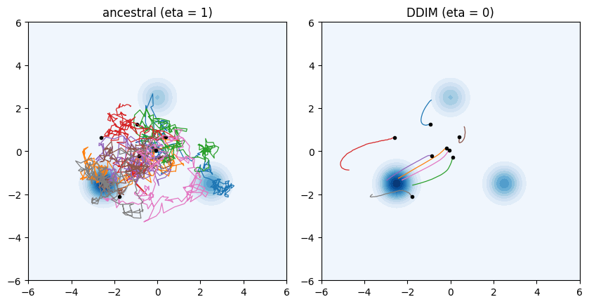
key, k1, k2 = jax.random.split(key, 3)
starts = jax.random.normal(k1, (8, 2))
_, path_ddpm = ddim_sample(net, starts, k2, 200, eta=1.0, record=True)
_, path_ddim = ddim_sample(net, starts, k2, 200, record=True)
axis = jnp.linspace(-6, 6, 121)
grid = jnp.stack(jnp.meshgrid(axis, axis, indexing='ij'), -1).reshape(-1, 2)
density = jnp.exp(mix.log_prob(grid)).reshape(121, 121).T
fig, axes = d2l.plt.subplots(1, 2, figsize=(8.5, 4.2))
for ax, path, title in zip(axes, (path_ddpm, path_ddim), ('ancestral (eta = 1)', 'DDIM (eta = 0)')):
    ax.contourf(axis, axis, density, levels=12, cmap='Blues')
    for i in range(8):
        ax.plot(path[:, i, 0], path[:, i, 1], lw=0.9)
        ax.plot(path[0, i, 0], path[0, i, 1], 'ko', ms=3)
    ax.set_title(title), ax.set_aspect('equal')
fig.tight_layout()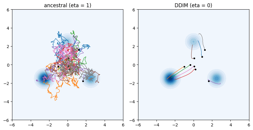
17.9.4 Fast Sampling for Images
The same sampler applies to the U-Net of Section 17.8. We train an unconditional model for a thousand updates, about seven minutes on a laptop processor, with the schedule of Ho et al. (2020) and the moving average of Section 17.8.
fmnist = d2l.FashionMNIST(batch_size=128)
X = fmnist.train.data.float()[:, None] / 255 * 2 - 1
T_img = 1000
beta_img = torch.linspace(1e-4, 0.02, T_img)
alpha_img = 1 - beta_img
alpha_bar_img = torch.cumprod(alpha_img, 0)

torch.manual_seed(5)
unet = d2l.UNet()
ema = d2l.UNet()
ema.load_state_dict(unet.state_dict())
optimizer = torch.optim.Adam(unet.parameters(), lr=1e-3)
for step in range(1000):
    x0 = X[torch.randint(0, len(X), (128,))]
    t = torch.randint(0, T_img, (128,))
    eps = torch.randn_like(x0)
    a = alpha_bar_img[t][:, None, None, None]
    loss = ((unet(a.sqrt() * x0 + (1 - a).sqrt() * eps, t) - eps) ** 2).mean()
    optimizer.zero_grad(), loss.backward(), optimizer.step()
    decay = min(0.999, (1 + step) / (10 + step))
    with torch.no_grad():
        for p_ema, p in zip(ema.parameters(), unet.parameters()):
            p_ema.mul_(decay).add_(p, alpha=1 - decay)
print(f'final training loss: {loss.item():.3f}')
final training loss: 0.039fmnist = d2l.FashionMNIST(batch_size=128)
X = jnp.asarray(fmnist.train[0], jnp.float32)[..., None] / 255 * 2 - 1
T_img = 1000
beta_img = jnp.linspace(1e-4, 0.02, T_img)
alpha_img = 1 - beta_img
alpha_bar_img = jnp.cumprod(alpha_img)
unet = d2l.UNet(rngs=nnx.Rngs(5))
graphdef, ema_state = nnx.split(unet)
optimizer = nnx.Optimizer(unet, optax.adam(1e-3), wrt=nnx.Param)
@nnx.jit
def unet_step(unet, optimizer, x0, t, eps):
def loss_fn(model):
a = alpha_bar_img[t][:, None, None, None]
return ((model(jnp.sqrt(a) * x0 + jnp.sqrt(1 - a) * eps, t) - eps) ** 2).mean()
loss, grads = nnx.value_and_grad(loss_fn)(unet)
optimizer.update(unet, grads)
return loss
@jax.jit
def ema_update(ema_state, state, decay):
return jax.tree_util.tree_map(lambda e, p: decay * e + (1 - decay) * p,
ema_state, state)
for step in range(1000):
key, k1, k2, k3 = jax.random.split(key, 4)
x0 = X[jax.random.randint(k1, (128,), 0, len(X))]
loss = unet_step(unet, optimizer, x0, jax.random.randint(k2, (128,), 0, T_img),
jax.random.normal(k3, x0.shape))
ema_state = ema_update(ema_state, nnx.state(unet),
min(0.999, (1 + step) / (10 + step)))
ema = nnx.merge(graphdef, ema_state)
print(f'final training loss: {loss:.3f}')final training loss: 0.048The image sampler is Equation 17.9.3 again, on the thousand-step schedule. We draw eight noise images once and generate from them three times: with the ancestral chain on all thousand steps, and with DDIM on fifty and on ten steps.
@torch.no_grad()
def ddim_images(model, x, steps, eta=0.0):
    taus = torch.linspace(T_img - 1, 0, steps).round().long().tolist()
    a_bars = [alpha_bar_img[t].item() for t in taus] + [1.0]
    for k, t in enumerate(taus):
        a_t, a_s = a_bars[k], a_bars[k + 1]
        eps = model(x, torch.full((len(x),), t))
        x0_hat = (x - (1 - a_t) ** 0.5 * eps) / a_t ** 0.5
        sigma = eta * ((1 - a_s) / (1 - a_t) * (1 - a_t / a_s)) ** 0.5 if a_s < 1 else 0
        x = (a_s ** 0.5 * x0_hat + max(1 - a_s - sigma ** 2, 0) ** 0.5 * eps
             + sigma * torch.randn_like(x))
    return x

torch.manual_seed(6)
x_T = torch.randn(8, 1, 28, 28)
rows = [ddim_images(ema, x_T, 1000, eta=1.0), ddim_images(ema, x_T, 50),
        ddim_images(ema, x_T, 10)]
print('rows: ancestral, 1000 steps | DDIM, 50 steps | DDIM, 10 steps')
imgs = torch.cat(rows).clamp(-1, 1) / 2 + 0.5
d2l.show_images(imgs.permute(0, 2, 3, 1).repeat(1, 1, 1, 3), 3, 8, scale=0.8);
rows: ancestral, 1000 steps | DDIM, 50 steps | DDIM, 10 steps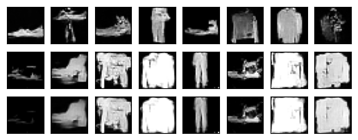
@nnx.jit
def ddim_image_step(model, x, t, a_t, a_s, sigma, key):
    eps = model(x, jnp.full((len(x),), t))
    x0_hat = (x - jnp.sqrt(1 - a_t) * eps) / jnp.sqrt(a_t)
    return (jnp.sqrt(a_s) * x0_hat + jnp.sqrt(jnp.maximum(1 - a_s - sigma ** 2, 0)) * eps
            + sigma * jax.random.normal(key, x.shape))

def ddim_images(model, x, key, steps, eta=0.0):
    taus = [int(t) for t in jnp.round(jnp.linspace(T_img - 1, 0, steps))]
    a_bars = [float(alpha_bar_img[t]) for t in taus] + [1.0]
    for k, t in enumerate(taus):
        a_t, a_s = a_bars[k], a_bars[k + 1]
        sigma = eta * ((1 - a_s) / (1 - a_t) * (1 - a_t / a_s)) ** 0.5 if a_s < 1 else 0.0
        key, subkey = jax.random.split(key)
        x = ddim_image_step(model, x, t, a_t, a_s, sigma, subkey)
    return x

key, k1, k2 = jax.random.split(key, 3)
x_T = jax.random.normal(k1, (8, 28, 28, 1))
rows = [ddim_images(ema, x_T, k2, 1000, eta=1.0), ddim_images(ema, x_T, k2, 50),
        ddim_images(ema, x_T, k2, 10)]
print('rows: ancestral, 1000 steps | DDIM, 50 steps | DDIM, 10 steps')
imgs = jnp.concatenate(rows).clip(-1, 1) / 2 + 0.5
d2l.show_images(jnp.repeat(imgs, 3, -1), 3, 8, scale=0.8);
rows: ancestral, 1000 steps | DDIM, 50 steps | DDIM, 10 steps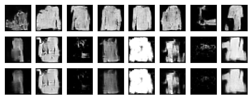
The second and third rows resemble each other column by column: both approximate the same deterministic map from \(\mathbf{x}_T\), the solution of the ODE above, ten steps more coarsely than fifty. The first row does not, because the ancestral chain injects fresh noise at every step; under that chain, as Song et al. (2021) note, the same \(\mathbf{x}_T\) leads to highly diverse samples. The deterministic rows cost a twentieth and a hundredth of the chain, but for this small network trained for a thousand updates they are also flatter in shading, and a few of their samples come out dark or saturated. The deterministic sampler exposes errors of the noise predictor that the stochastic one partly corrects. Each stochastic step contains a Langevin-like component, an extra step along the score together with fresh noise, that pulls the state toward the model’s marginal at that level and so corrects errors made at earlier steps (Karras et al. 2022). The deterministic update carries every error forward. Song et al. (2021) report that fifty steps approach the chain’s sample quality for well-trained predictors; this predictor, trained for a thousand updates, does not reach that point. The latent code is meaningful for the deterministic sampler regardless, and interpolating between two codes interpolates between two images. The cell interpolates along the great circle between two noise images, which keeps the norm of the code close to that of its endpoints, the norm typical of Gaussian noise images, whereas a straight line would shrink it in the middle; it decodes each point with fifty DDIM steps.
torch.manual_seed(7)
z0, z1 = torch.randn(2, 1, 28, 28)
angle = torch.acos((z0 * z1).sum() / (z0.norm() * z1.norm()))
lam = torch.linspace(0, 1, 8)
codes = torch.stack([(torch.sin((1 - l) * angle) * z0 + torch.sin(l * angle) * z1)
                     / torch.sin(angle) for l in lam])
imgs = ddim_images(ema, codes, 50).clamp(-1, 1) / 2 + 0.5
d2l.show_images(imgs.permute(0, 2, 3, 1).repeat(1, 1, 1, 3), 1, 8, scale=0.8);
key, k1, k2 = jax.random.split(key, 3)
z0, z1 = jax.random.normal(k1, (2, 28, 28, 1))
angle = jnp.arccos((z0 * z1).sum() / (jnp.linalg.norm(z0) * jnp.linalg.norm(z1)))
lam = jnp.linspace(0, 1, 8)
codes = jnp.stack([(jnp.sin((1 - l) * angle) * z0 + jnp.sin(l * angle) * z1)
                   / jnp.sin(angle) for l in lam])
imgs = ddim_images(ema, codes, k2, 50).clip(-1, 1) / 2 + 0.5
d2l.show_images(jnp.repeat(imgs, 3, -1), 1, 8, scale=0.8);
The images change gradually along the row, from the image decoded at one code to the image decoded at the other through intermediate shapes; either endpoint can be one of this small model’s failed samples. The gradual change is possible because the sampler is a continuous function of its code. A related property underlies DDIM inversion: running the deterministic update forward from a real image recovers a code that approximately regenerates it (Song et al. 2021), a starting point for editing the image through its code.
17.9.5 Summary
The DDPM training objective constrains only the marginals \(q(\mathbf{x}_t \mid \mathbf{x}_0)\), and the non-Markovian family Equation 17.9.1 shares those marginals for every choice of the noise scales \(\sigma_t\), so one trained noise predictor serves the whole family. Its reverse update Equation 17.9.3 predicts the clean point, re-noises it to the next level along the predicted noise direction, and adds noise of scale \(\sigma_t\); \(\eta = 1\) on the full grid of steps recovers the DDPM chain with its posterior variance, and \(\eta = 0\) gives the deterministic DDIM. Because the marginals do not depend on step spacing, the sampler can skip steps, at a cost that grows with the stride and that the running example measured exactly with the optimal predictor.
On the mixture, fifty deterministic steps reproduced the statistics of two hundred, and on Fashion-MNIST fifty steps produced garment-like images at a twentieth of the cost of the chain, with the small model’s errors more visible than under the stochastic sampler. Determinism makes the noise image a latent code: the same code gives closely resembling samples under different step counts, and interpolated codes give interpolated images. In the small-step limit the update integrates an ordinary differential equation, which places DDIM in the continuous-time picture of the next section and of Section 29.4.
17.9.6 Exercises
- The Markov member. Show that choosing \(\sigma_t^2 = \tilde{\beta}_t\) in Equation 17.9.1 makes \(q_\sigma(\mathbf{x}_{t-1} \mid \mathbf{x}_t, \mathbf{x}_0)\) equal to the DDPM posterior Equation 17.7.7, by rewriting the mean of Equation 17.9.1 in terms of \(\mathbf{x}_0\) and \(\mathbf{x}_t\) and comparing coefficients. Conclude that the process is then Markov with the DDPM transitions.
- The last step. The sampler treats the transition from the smallest retained step to the clean point by returning \(\hat{\mathbf{x}}_0\). Show that this is Equation 17.9.3 with \(\bar{\alpha}_{t-1} = 1\), and explain why no noise is added there for any \(\eta\).
- Bound and weights. Song et al. (2021) show that the variational bound of the non-Markovian model equals a weighted noise-prediction objective plus a constant. Starting from Equation 17.7.11, explain why a network that minimizes the unweighted simple loss for every \(t\) separately also minimizes every weighted version, provided its capacity does not tie the steps together. What does this argument assume about the network?
- [code] The strength \(\eta\). Sample the running example with \(\eta \in \{0, 0.25, 0.5, 1\}\) on twenty steps and on two hundred, and report the summary statistics. At which step count does the stochastic sampler have the advantage, and which statistic reveals it?
- [code] Consistency across step counts. For the image model, generate from the same eight codes with DDIM on \(10\), \(20\), \(50\), and \(100\) steps, and measure the mean squared distance between the fifty-step images and each of the others. Then repeat with \(\eta = 1\). Which sampler produces images that converge as the step count grows, and why?
- [code] Inversion. Run the deterministic update in the forward direction on a test image, from step \(0\) to step \(T\), using the predicted noise at each step to re-noise, and then regenerate from the resulting code with the same number of steps. Measure the reconstruction error as a function of the number of steps and explain its source.