%matplotlib inline
from d2l import torch as d2l
import torch
from torch import nn17.3 Score Matching
Maximum likelihood requires samples from the model at every update because the gradient of the log-partition function is a model expectation. This section replaces the likelihood with an objective whose gradient involves only data. The objective compares not densities but the gradients of their logarithms with respect to the input, and it can be rewritten, by an integration by parts, into a form that contains no unknown quantity. The resulting method, score matching, was introduced by Hyvärinen (2005) for the purpose of fitting unnormalized models; its role in generative modeling was established by Song and Ermon (2019). The presentation follows lecture 12 of Kuleshov (2023) .
%matplotlib inline
from d2l import jax as d2l
import jax
from jax import numpy as jnp
from flax import nnx
import optax
17.3.1 The Score Function
For a differentiable density \(p\) on \(\mathbb{R}^d\), the score is the gradient of the log-density with respect to the input,
\[ \nabla_{\mathbf{x}} \log p(\mathbf{x}) : \mathbb{R}^d \to \mathbb{R}^d . \]
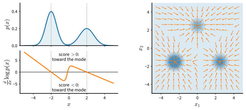
The score is a vector field. At each point it gives the direction in which the density increases fastest and the rate of that increase on the logarithmic scale. This gradient is taken with respect to the input \(\mathbf{x}\), not the parameters, and it should be distinguished from the parameter gradient \(\nabla_{\boldsymbol{\theta}} \log p_{\boldsymbol{\theta}}(\mathbf{x})\) that maximum likelihood uses; both are historically called scores, and the input gradient is sometimes called the Stein score to keep them apart. Figure 17.3.1 shows the score of a bimodal density in one dimension, where it is a signed slope, and of the chapter’s running example, the Gaussian mixture of Section 17.2, in two, where it is a field of arrows pointing toward the modes (Section 29.3.4 develops the same object for continuous-time dynamics).
For an energy-based model the score is available without the normalizer. Taking the gradient of \(\log p_{\boldsymbol{\theta}}(\mathbf{x}) = -E_{\boldsymbol{\theta}}(\mathbf{x}) - \log Z(\boldsymbol{\theta})\) removes the second term, which does not depend on \(\mathbf{x}\):
\[ \nabla_{\mathbf{x}} \log p_{\boldsymbol{\theta}}(\mathbf{x}) = -\nabla_{\mathbf{x}} E_{\boldsymbol{\theta}}(\mathbf{x}). \tag{17.3.1}\]
This observation suggests changing what is learned. Instead of fitting the density and struggling with \(Z(\boldsymbol{\theta})\), fit the score of the data distribution with a model \(\mathbf{s}_{\boldsymbol{\theta}}: \mathbb{R}^d \to \mathbb{R}^d\). The model can be the negative gradient of an energy network, \(-\nabla_{\mathbf{x}} E_{\boldsymbol{\theta}}\), in which case it is automatically the score of an energy-based model, or an arbitrary network with \(d\) outputs, which is simpler to train and is the choice made below. A general vector field need not be the gradient of any function, so the second choice gives up the guarantee that a density exists whose score is \(\mathbf{s}_{\boldsymbol{\theta}}\). The samplers of the following sections use only the field, so what matters for them is how close the field is to the true score, not whether it is exactly the gradient of some function. The training set is a sample \(\mathbf{x}_1, \ldots, \mathbf{x}_n\) from \(p\), and the goal is \(\mathbf{s}_{\boldsymbol{\theta}}(\mathbf{x}) \approx \nabla_{\mathbf{x}} \log p(\mathbf{x})\).
17.3.2 The Fisher Divergence
A model score should agree with the data score wherever the data are. The natural measure of disagreement between two vector fields is the average squared distance between them under the data distribution,
\[ J_{\textrm{ESM}}(\boldsymbol{\theta}) = \frac{1}{2}\, \mathbb{E}_{\mathbf{x} \sim p} \left[\, \big\| \mathbf{s}_{\boldsymbol{\theta}}(\mathbf{x}) - \nabla_{\mathbf{x}} \log p(\mathbf{x}) \big\|^2 \right], \tag{17.3.2}\]
the Fisher divergence between the data and the model (Section 28.2.4.1), also called the explicit score matching objective. It is zero exactly when the two fields agree at almost every point that the data can occupy. If \(\mathbf{s}_{\boldsymbol{\theta}}\) is itself the score of a density \(q_{\boldsymbol{\theta}}\) and both densities are positive on all of \(\mathbb{R}^d\), equal scores mean that \(\log q_{\boldsymbol{\theta}}\) and \(\log p\) differ by a constant, and because both densities integrate to one, the constant is zero: minimizing the Fisher divergence to zero recovers the data distribution. The objective never mentions \(Z(\boldsymbol{\theta})\). It does mention \(\nabla_{\mathbf{x}} \log p\), the score of the data distribution, which is the quantity we do not have.
17.3.3 Hyvärinen’s Identity
The unknown score can be removed. Expanding the square in Equation 17.3.2 gives three terms: \(\tfrac12 \mathbb{E}\|\nabla \log p\|^2\), which does not depend on \(\boldsymbol{\theta}\) and can be ignored during optimization; \(\tfrac12 \mathbb{E}\|\mathbf{s}_{\boldsymbol{\theta}}\|^2\), which is computable from samples; and the cross term \(-\mathbb{E}[\mathbf{s}_{\boldsymbol{\theta}}^\top \nabla \log p]\), which contains the unknown. In one dimension the cross term becomes computable after an integration by parts:
\[ -\int s_{\boldsymbol{\theta}}(x)\, \frac{p'(x)}{p(x)}\, p(x)\, dx = -\int s_{\boldsymbol{\theta}}(x)\, p'(x)\, dx = -\big[ s_{\boldsymbol{\theta}}(x)\, p(x) \big]_{-\infty}^{\infty} + \int s_{\boldsymbol{\theta}}'(x)\, p(x)\, dx = \mathbb{E}_{x \sim p}\big[ s_{\boldsymbol{\theta}}'(x) \big]. \]
The first equality cancels \(p\) against the denominator of the score, and the boundary term vanishes because \(p(x)\, s_{\boldsymbol{\theta}}(x) \to 0\) as \(|x| \to \infty\), an assumption that holds for any density with sufficiently light tails and any model that does not grow faster than they decay. The derivative has moved from the unknown density onto the model. In \(d\) dimensions the same step applies to each coordinate and the derivatives add up to the divergence of the field. The result is Hyvärinen’s identity:
\[ J_{\textrm{ESM}}(\boldsymbol{\theta}) = \mathbb{E}_{\mathbf{x} \sim p} \left[\, \frac{1}{2} \big\| \mathbf{s}_{\boldsymbol{\theta}}(\mathbf{x}) \big\|^2 + \operatorname{tr}\big( \nabla_{\mathbf{x}} \mathbf{s}_{\boldsymbol{\theta}}(\mathbf{x}) \big) \right] + \frac{1}{2}\, \mathbb{E}_{\mathbf{x} \sim p} \big\| \nabla_{\mathbf{x}} \log p(\mathbf{x}) \big\|^2, \tag{17.3.3}\]
where \(\nabla_{\mathbf{x}} \mathbf{s}_{\boldsymbol{\theta}}\) is the \(d \times d\) Jacobian of the model and its trace is \(\sum_i \partial s_{\boldsymbol{\theta}, i} / \partial x_i\). The proof with its regularity conditions is given in Section 29.4.1 (Equation 29.4.2). The last term is a constant, so the score matching objective is the expectation in the middle, and it is an average over data of quantities computed from the model alone. Its two terms have opposite tendencies. The squared norm keeps the field small. The trace rewards negative divergence at the data, the property of a field that converges on them from all sides. Together they favor a field that points toward higher density and vanishes at the modes, which is what a score looks like near a mode.
17.3.3.1 Verifying the Identity
The identity can be checked on the running example because its score is known. The cell evaluates the score matching objective at the true score, by automatic differentiation of the closed-form field, on two hundred thousand samples; adding the constant should give the Fisher divergence of the true score with itself, which is zero. The model class is a small multilayer perceptron with two outputs, and the helper computes the Fisher divergence of any score model against the truth on a given set of points.
torch.manual_seed(0)
mix = d2l.GaussianMixture(means=[[-2.5, -1.5], [2.5, -1.5], [0.0, 2.5]],
                          weights=[0.5, 0.3, 0.2], std=0.5)
data, test = mix.sample(2000), mix.sample(2000)

class ScoreNet(nn.Module):
    """A two-dimensional score model: a multilayer perceptron with two outputs."""
    def __init__(self, hidden=128):
        super().__init__()
        self.net = nn.Sequential(nn.Linear(2, hidden), nn.SiLU(),
                                 nn.Linear(hidden, hidden), nn.SiLU(),
                                 nn.Linear(hidden, 2))

    def forward(self, x):
        return self.net(x)

def fisher_divergence(score, x):
    """0.5 E||s(x) - grad log p(x)||^2 on the given points."""
    with torch.no_grad():
        return 0.5 * ((score(x) - mix.score(x)) ** 2).sum(1).mean().item()

def score_matching_loss(score, x):
    """Hyvarinen's objective E[0.5 ||s||^2 + tr(ds/dx)], trace by autograd."""
    x = x.clone().requires_grad_(True)
    s = score(x)
    # trace = sum_i ds_i/dx_i: the gradient of the batch sum of s_i with respect
    # to x has row b equal to ds_i(x_b)/dx_b, of which entry i is the diagonal term
    trace = sum(torch.autograd.grad(s[:, i].sum(), x, create_graph=True)[0][:, i]
                for i in range(x.shape[1]))
    return (0.5 * (s ** 2).sum(1) + trace).mean()

def objective_on(score, x, chunk=20_000):  # average over a large sample
    return sum(score_matching_loss(score, c).item() * len(c)
               for c in x.split(chunk)) / len(x)

torch.manual_seed(1)
big = mix.sample(200_000)
const = 0.5 * (mix.score(big) ** 2).sum(1).mean().item()
objective = objective_on(mix.score, big)
print(f'objective at the true score: {objective:.3f}, '
      f'constant: {const:.3f}, sum: {objective + const:.3f}')
objective at the true score: -3.988, constant: 4.012, sum: 0.024key = jax.random.PRNGKey(0)
mix = d2l.GaussianMixture(means=[[-2.5, -1.5], [2.5, -1.5], [0.0, 2.5]],
weights=[0.5, 0.3, 0.2], std=0.5)
key, k1, k2 = jax.random.split(key, 3)
data, test = mix.sample(k1, 2000), mix.sample(k2, 2000)
class ScoreNet(nnx.Module):
"""A two-dimensional score model: a multilayer perceptron with two outputs."""
def __init__(self, hidden=128, rngs=None):
self.h1 = nnx.Linear(2, hidden, rngs=rngs)
self.h2 = nnx.Linear(hidden, hidden, rngs=rngs)
self.out = nnx.Linear(hidden, 2, rngs=rngs)
def __call__(self, x):
return self.out(nnx.silu(self.h2(nnx.silu(self.h1(x)))))
def fisher_divergence(score, x):
"""0.5 E||s(x) - grad log p(x)||^2 on the given points."""
return float(0.5 * ((score(x) - mix.score(x)) ** 2).sum(1).mean())
def score_matching_loss(score, x):
"""Hyvarinen's objective E[0.5 ||s||^2 + tr(ds/dx)], trace by autodiff."""
s = score(x)
f = lambda q: score(q[None])[0] # the field at a single point, for its Jacobian
trace = jax.vmap(lambda q: jnp.trace(jax.jacfwd(f)(q)))(x)
return (0.5 * (s ** 2).sum(1) + trace).mean()
def objective_on(score, x, chunks=10): # average over a large sample
return float(sum(score_matching_loss(score, c)
for c in jnp.array_split(x, chunks)) / chunks)
key, subkey = jax.random.split(key)
big = mix.sample(subkey, 200_000)
const = float(0.5 * (mix.score(big) ** 2).sum(1).mean())
objective = objective_on(mix.score, big)
print(f'objective at the true score: {objective:.3f}, '
f'constant: {const:.3f}, sum: {objective + const:.3f}')objective at the true score: -4.005, constant: 3.994, sum: -0.011The objective at the true score is about \(-4\), the constant is about \(+4\), and the sum vanishes to within the Monte Carlo error of the average. The two terms of the objective are large individually, of opposite sign, and cancel at the optimum. This cancellation is also why estimates of the Fisher divergence from a few thousand points are noisy: the per-point value of \(\tfrac12 \|\mathbf{s}\|^2 + \operatorname{tr}(\nabla_{\mathbf{x}} \mathbf{s}) + \tfrac12 \|\nabla_{\mathbf{x}} \log p\|^2\), whose average the cell reports as the sum, has a standard deviation of about eight, so its average over two thousand points is uncertain by about \(0.2\), and over two hundred thousand by about \(0.02\).
17.3.3.2 Training by Exact Score Matching
The objective with the trace is called implicit score matching, because the data score enters only implicitly, through the integration by parts; the subscript ESM of Equation 17.3.2 stands for explicit score matching, the objective written with the data score. We call its minimization with the trace computed exactly exact score matching, to distinguish it from the sliced estimate below. In two dimensions the trace costs one extra derivative pass per input coordinate, so the loop below runs in seconds. After training, the Fisher divergence on the test points reports the fit against the true score, and the large sample checks the identity again, this time for the learned field: the objective plus the constant should agree with the directly computed Fisher divergence.
def train(loss_fn, steps=2000, lr=1e-3, seed=1):
    torch.manual_seed(seed)
    score = ScoreNet()
    optimizer = torch.optim.Adam(score.parameters(), lr=lr)
    for step in range(steps):
        x = data[torch.randint(0, len(data), (256,))]
        loss = loss_fn(score, x)
        optimizer.zero_grad(), loss.backward(), optimizer.step()
    return score

score_exact = train(score_matching_loss)
print(f'exact score matching: Fisher divergence on the test points '
      f'{fisher_divergence(score_exact, test):.3f}')
print(f'on 200,000 samples: objective + constant '
      f'{objective_on(score_exact, big) + const:.3f}, '
      f'direct Fisher divergence {fisher_divergence(score_exact, big):.3f}')
exact score matching: Fisher divergence on the test points 0.089
on 200,000 samples: objective + constant 0.107, direct Fisher divergence 0.086def train(step_fn, key, steps=2000, lr=1e-3, seed=1):
score = ScoreNet(rngs=nnx.Rngs(seed))
optimizer = nnx.Optimizer(score, optax.adam(lr), wrt=nnx.Param)
for step in range(steps):
key, k1, k2 = jax.random.split(key, 3)
x = data[jax.random.randint(k1, (256,), 0, len(data))]
step_fn(score, optimizer, x, k2)
return score
@nnx.jit
def exact_step(score, optimizer, x, key):
loss, grads = nnx.value_and_grad(score_matching_loss)(score, x)
optimizer.update(score, grads)
return loss
key, subkey = jax.random.split(key)
score_exact = train(exact_step, subkey)
print(f'exact score matching: Fisher divergence on the test points '
f'{fisher_divergence(score_exact, test):.3f}')
print(f'on 200,000 samples: objective + constant '
f'{objective_on(score_exact, big) + const:.3f}, '
f'direct Fisher divergence {fisher_divergence(score_exact, big):.3f}')exact score matching: Fisher divergence on the test points 0.118
on 200,000 samples: objective + constant 0.116, direct Fisher divergence 0.125The learned field is within about a tenth of the true score in Fisher divergence, on a target whose score has a mean squared norm of about eight, and the two ways of computing the divergence agree to within their Monte Carlo error. Nothing in the training loop used the density, its normalizer, or a sample from the model. The model class is saved to the d2l library as ScoreNet, since the next two sections train it again.
The trace prevents this loop from scaling. For an input of dimension \(d\), the trace of the Jacobian needs \(d\) derivative passes through the network per training example, or a Jacobian-vector product per coordinate (Section 25.3), because automatic differentiation delivers one row or one column of the Jacobian at a time. Two coordinates cost two passes; an image with a hundred thousand pixels would cost a hundred thousand. Two remedies follow. Sliced score matching, next, estimates the trace with random projections. Denoising score matching, the subject of Section 17.4, changes the target so that no Jacobian appears at all.
17.3.4 Sliced Score Matching
The expensive quantity is a trace, and a trace can be estimated by random projection: for any matrix \(A\) and a random vector \(\mathbf{v}\) with \(\mathbb{E}[\mathbf{v} \mathbf{v}^\top] = I\), one has \(\mathbb{E}[\mathbf{v}^\top A \mathbf{v}] = \operatorname{tr}(A)\). Song et al. (2019) build the estimator into the objective from the start. Instead of matching the full vector fields, match their projections onto random directions. The sliced Fisher divergence is
\[ \frac{1}{2}\, \mathbb{E}_{\mathbf{v} \sim p_{\mathbf{v}}}\, \mathbb{E}_{\mathbf{x} \sim p} \left[ \big( \mathbf{v}^\top \mathbf{s}_{\boldsymbol{\theta}}(\mathbf{x}) - \mathbf{v}^\top \nabla_{\mathbf{x}} \log p(\mathbf{x}) \big)^2 \right], \tag{17.3.4}\]
where \(p_{\mathbf{v}}\) is a distribution over projection vectors with \(\mathbb{E}[\mathbf{v} \mathbf{v}^\top] = I\), typically standard Gaussian or uniform on the sign vectors \(\{-1, +1\}^d\). It vanishes exactly when the fields agree, because averaging the squared projection of a vector \(\mathbf{a}\) over such directions gives \(\mathbf{a}^\top \mathbb{E}[\mathbf{v} \mathbf{v}^\top]\, \mathbf{a} = \|\mathbf{a}\|^2\). The integration by parts of the previous section, applied to the scalar field \(\mathbf{v}^\top \mathbf{s}_{\boldsymbol{\theta}}\) along the direction \(\mathbf{v}\), replaces the cross term \(\mathbb{E}[(\mathbf{v}^\top \mathbf{s}_{\boldsymbol{\theta}})(\mathbf{v}^\top \nabla_{\mathbf{x}} \log p)]\) by \(-\mathbb{E}[\mathbf{v}^\top (\nabla_{\mathbf{x}} \mathbf{s}_{\boldsymbol{\theta}}) \mathbf{v}]\), the derivative of \(\mathbf{v}^\top \mathbf{s}_{\boldsymbol{\theta}}\) along \(\mathbf{v}\); this removes the data score and gives the sliced score matching objective
\[ J_{\textrm{SSM}}(\boldsymbol{\theta}) = \mathbb{E}_{\mathbf{v} \sim p_{\mathbf{v}}}\, \mathbb{E}_{\mathbf{x} \sim p} \left[ \mathbf{v}^\top \nabla_{\mathbf{x}} \mathbf{s}_{\boldsymbol{\theta}}(\mathbf{x})\, \mathbf{v} + \frac{1}{2} \big( \mathbf{v}^\top \mathbf{s}_{\boldsymbol{\theta}}(\mathbf{x}) \big)^2 \right], \tag{17.3.5}\]
up to a constant. The first term is a directional derivative of a scalar, the derivative of \(\mathbf{v}^\top \mathbf{s}_{\boldsymbol{\theta}}\) along \(\mathbf{v}\), and costs one derivative pass regardless of \(d\). With one random direction per training point, the cost of a sliced update is a small constant multiple of the cost of a forward pass. When \(\mathbb{E}[\mathbf{v} \mathbf{v}^\top] = I\), averaging over \(\mathbf{v}\) recovers both the trace and \(\tfrac12 \|\mathbf{s}_{\boldsymbol{\theta}}\|^2\), so the sliced objective equals Equation 17.3.3 up to the constant. Replacing \(\tfrac12 (\mathbf{v}^\top \mathbf{s}_{\boldsymbol{\theta}})^2\) by its exact average \(\tfrac12 \|\mathbf{s}_{\boldsymbol{\theta}}\|^2\) removes one random term; the original paper calls this variant SSM-VR and found that it performed better in its experiments, although the replacement is not guaranteed to lower the variance (Exercise 5). Song et al. (2019) prove that, for a well-specified parametric model of the density, the estimator is consistent and asymptotically normal under standard regularity conditions. The cost is variance: each update sees the Jacobian through one random direction. The cell below computes \(\mathbf{v}^\top (\nabla_{\mathbf{x}} \mathbf{s}_{\boldsymbol{\theta}}) \mathbf{v}\) as the derivative of the scalar \(\mathbf{v}^\top \mathbf{s}_{\boldsymbol{\theta}}\) along \(\mathbf{v}\), one derivative pass per point (a Jacobian-vector product in JAX, the equivalent vector-Jacobian product in PyTorch), and adds \(\tfrac12 (\mathbf{v}^\top \mathbf{s}_{\boldsymbol{\theta}})^2\).
def sliced_score_matching_loss(score, x):
    """E_v[v^T (ds/dx) v + 0.5 (v^T s)^2], one Gaussian direction per point."""
    x = x.clone().requires_grad_(True)
    v = torch.randn_like(x)
    s = score(x)
    jv = torch.autograd.grad((s * v).sum(), x, create_graph=True)[0]  # J^T v
    return ((v * jv).sum(1) + 0.5 * (s * v).sum(1) ** 2).mean()

score_sliced = train(sliced_score_matching_loss)
print(f'sliced score matching: Fisher divergence on the test points '
      f'{fisher_divergence(score_sliced, test):.3f}')
sliced score matching: Fisher divergence on the test points 0.083def sliced_score_matching_loss(score, x, v):
"""E_v[v^T (ds/dx) v + 0.5 (v^T s)^2], one Gaussian direction per point."""
f = lambda q: score(q[None])[0]
s, jv = jax.vmap(lambda q, u: jax.jvp(f, (q,), (u,)))(x, v) # s and J v
return ((v * jv).sum(1) + 0.5 * (s * v).sum(1) ** 2).mean()
@nnx.jit
def sliced_step(score, optimizer, x, key):
v = jax.random.normal(key, x.shape)
loss, grads = nnx.value_and_grad(sliced_score_matching_loss)(score, x, v)
optimizer.update(score, grads)
return loss
key, subkey = jax.random.split(key)
score_sliced = train(sliced_step, subkey)
print(f'sliced score matching: Fisher divergence on the test points '
f'{fisher_divergence(score_sliced, test):.3f}')sliced score matching: Fisher divergence on the test points 0.115The sliced estimator reaches a Fisher divergence comparable to the exact one after the same number of updates, each of which was cheaper. The three panels below compare the true field with the two learned fields over the plane, with training points in grey. Arrows longer than a fixed length are clipped so that the directions remain visible far from the data, where the true score is large.
g = torch.linspace(-4.5, 4.5, 16)
pts = torch.stack(torch.meshgrid(g, g, indexing='ij'), -1).reshape(-1, 2)
with torch.no_grad():
    fields = [('true score', mix.score(pts)),
              ('exact score matching', score_exact(pts)),
              ('sliced score matching', score_sliced(pts))]
fig, axes = d2l.plt.subplots(1, 3, figsize=(10.5, 3.6))
for ax, (title, f) in zip(axes, fields):
    f = f * torch.clamp(2 / f.norm(dim=1, keepdim=True), max=1)  # clip length
    ax.scatter(data[:500, 0], data[:500, 1], s=3, c='lightgray')
    ax.quiver(pts[:, 0], pts[:, 1], f[:, 0], f[:, 1], angles='xy',
              scale_units='xy', scale=2.5, width=0.005)
    ax.set_title(title), ax.set_aspect('equal')
fig.tight_layout()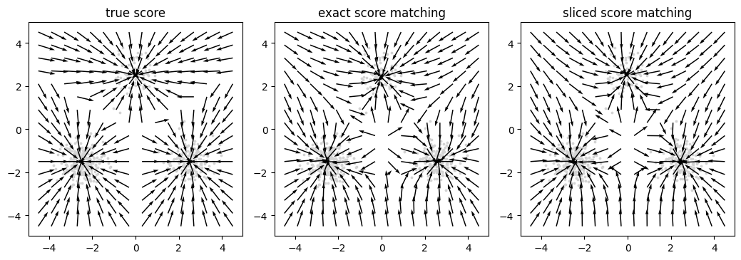
g = jnp.linspace(-4.5, 4.5, 16)
pts = jnp.stack(jnp.meshgrid(g, g, indexing='ij'), -1).reshape(-1, 2)
fields = [('true score', mix.score(pts)),
          ('exact score matching', score_exact(pts)),
          ('sliced score matching', score_sliced(pts))]
fig, axes = d2l.plt.subplots(1, 3, figsize=(10.5, 3.6))
for ax, (title, f) in zip(axes, fields):
    norm = jnp.linalg.norm(f, axis=1, keepdims=True)
    f = f * jnp.minimum(2 / norm, 1)  # clip the arrow length
    ax.scatter(data[:500, 0], data[:500, 1], s=3, c='lightgray')
    ax.quiver(pts[:, 0], pts[:, 1], f[:, 0], f[:, 1], angles='xy',
              scale_units='xy', scale=2.5, width=0.005)
    ax.set_title(title), ax.set_aspect('equal')
fig.tight_layout()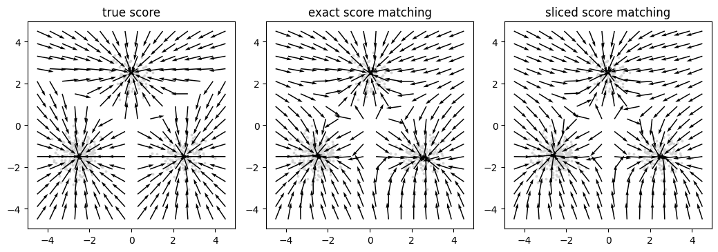
Near the three modes, all three fields agree: arrows converge on each component mean. Away from the data the learned fields differ from the truth in places. In the region between the modes, and toward the edges of the plot, the true field points toward the modes while some learned arrows point in directions that the training data never constrained; in two dimensions most of them still point roughly inward, and the table below quantifies how much accuracy is lost.
17.3.5 Where the Estimate Is Accurate
The objective is an expectation under the data distribution, so it constrains the field only where the data have appreciable density. The cell groups the points of a grid by the true log-density and reports, for each group, the mean squared error of the exact-score-matching field divided by the mean squared norm of the true score, a relative error that accounts for the score growing large in the tails.
axis = torch.linspace(-5, 5, 41)
grid = torch.stack(torch.meshgrid(axis, axis, indexing='ij'), -1).reshape(-1, 2)
with torch.no_grad():
    true_s, log_p = mix.score(grid), mix.log_prob(grid)
    err = ((score_exact(grid) - true_s) ** 2).sum(1)
print(f'{"log density":>13} {"grid points":>12} {"relative score error":>21}')
for lo, hi in ((-2, 0), (-4, -2), (-8, -4), (-16, -8), (-40, -16)):
    m = (log_p >= lo) & (log_p < hi)
    rel = err[m].mean() / (true_s[m] ** 2).sum(1).mean()
    print(f'[{lo:>4}, {hi:>4}) {m.sum().item():>12d} {rel:>21.3f}')
log density grid points relative score error
[ -2, 0) 30 0.018
[ -4, -2) 145 0.016
[ -8, -4) 308 0.049
[ -16, -8) 557 0.180
[ -40, -16) 547 0.122axis = jnp.linspace(-5, 5, 41)
grid = jnp.stack(jnp.meshgrid(axis, axis, indexing='ij'), -1).reshape(-1, 2)
true_s, log_p = mix.score(grid), mix.log_prob(grid)
err = ((score_exact(grid) - true_s) ** 2).sum(1)
print(f'{"log density":>13} {"grid points":>12} {"relative score error":>21}')
for lo, hi in ((-2, 0), (-4, -2), (-8, -4), (-16, -8), (-40, -16)):
m = (log_p >= lo) & (log_p < hi)
rel = err[m].mean() / (true_s[m] ** 2).sum(1).mean()
print(f'[{lo:>4}, {hi:>4}) {int(m.sum()):>12d} {rel:>21.3f}') log density grid points relative score error
[ -2, 0) 30 0.068
[ -4, -2) 145 0.024
[ -8, -4) 308 0.034
[ -16, -8) 557 0.154
[ -40, -16) 547 0.134In the two highest-density bands, roughly the region that contains most of the training data, the relative error is under ten percent. It rises to roughly ten to twenty percent in the two lowest bands, where the density is about three or more orders of magnitude below its peak. The estimate is accurate where the data are and unreliable elsewhere, which is what an objective weighted by the data density produces. This limitation is invisible while the model is only evaluated on data. It matters once a sampler starts from random noise, far from every mode, and must follow the field back to the data. Section 17.5 measures the effect in two dimensions, where it is mild, and explains why Song and Ermon (2019) expect it to be severe for images. The next section introduces the device that addresses both the cost of the trace and the emptiness of the low-density regions: perturbing the data with noise.
17.3.6 Summary
The score, the input gradient of the log-density, is free of the normalizer: for an energy-based model it is minus the gradient of the energy. Fitting a score model by the Fisher divergence Equation 17.3.2 would require the data score, but Hyvärinen’s identity Equation 17.3.3 rewrites the divergence, up to a constant, as the data expectation of \(\tfrac12 \|\mathbf{s}_{\boldsymbol{\theta}}\|^2 + \operatorname{tr}(\nabla_{\mathbf{x}} \mathbf{s}_{\boldsymbol{\theta}})\), which involves only the model. Training needs no samples from the model and no partition function. On the running example the identity was verified numerically and the learned field matched the true score to within about a tenth in Fisher divergence.
The trace of the Jacobian costs one derivative pass per input dimension. Sliced score matching Equation 17.3.5 replaces it with the derivative of \(\mathbf{v}^\top \mathbf{s}_{\boldsymbol{\theta}}\) along a random direction \(\mathbf{v}\), an unbiased estimate at constant cost per update, and reached a comparable fit in the experiment. The estimate is accurate only where the data density is appreciable: the relative error of the learned score rises to ten to twenty percent where the density is about three or more orders of magnitude below its peak.
17.3.7 Exercises
- Scores of standard densities. Compute the score of the Gaussian \(\mathcal{N}(\boldsymbol{\mu}, \Sigma)\), of the Laplace density \(\tfrac12 e^{-|x|}\), and of the mixture \(\sum_k \pi_k \mathcal{N}(\mathbf{x}; \boldsymbol{\mu}_k, \sigma^2 I)\). For the mixture, show that the score is the responsibility-weighted average of the component scores, which is what
GaussianMixture.scoreimplements. Where is the Laplace score undefined, and what does this imply for score matching on data with sharp features? - The identity in \(d\) dimensions. Carry out the integration by parts of the cross term coordinate by coordinate and derive Equation 17.3.3, stating explicitly the boundary condition used in each coordinate. Then show that for the model \(\mathbf{s}_{\boldsymbol{\theta}} = -\nabla_{\mathbf{x}} E_{\boldsymbol{\theta}}\) the trace term becomes minus the Laplacian of the energy, and interpret the sign: which energies does the objective favor at the data?
- Score matching for a Gaussian. Let the model be \(\mathbf{s}_{\boldsymbol{\theta}}(\mathbf{x}) = -A(\mathbf{x} - \mathbf{b})\) with \(A\) symmetric positive definite, the score of a Gaussian with precision \(A\). Write the score matching objective in closed form in terms of the sample mean and covariance of the data, minimize it, and show that the solution coincides with the maximum-likelihood estimate.
- The projection identity. Show that \(\mathbb{E}[\mathbf{v}^\top A \mathbf{v}] = \operatorname{tr}(A)\) whenever \(\mathbb{E}[\mathbf{v} \mathbf{v}^\top] = I\), and compute the variance of \(\mathbf{v}^\top A \mathbf{v}\) for a standard Gaussian \(\mathbf{v}\) and for a Rademacher (random sign) \(\mathbf{v}\) when \(A\) is symmetric. Which distribution gives the lower variance, and by how much when \(A\) is diagonal?
- [code] Variance reduction. Replace \(\tfrac12 (\mathbf{v}^\top \mathbf{s}_{\boldsymbol{\theta}})^2\) in Equation 17.3.5 by \(\tfrac12 \|\mathbf{s}_{\boldsymbol{\theta}}\|^2\) and retrain. Compare the Fisher divergence on the test points across five seeds for the two variants, and also try Rademacher projections. Report the mean and spread, and relate the differences to the variances computed in the previous exercise.
- [code] A conservative score model. Parameterize the score as the gradient of a scalar energy network, \(\mathbf{s}_{\boldsymbol{\theta}} = -\nabla_{\mathbf{x}} E_{\boldsymbol{\theta}}\), using automatic differentiation inside the forward pass, and train it by exact score matching. Compare its Fisher divergence with the unconstrained field, then use the learned energy to compute the log-density on the grid of Section 17.2 (normalizing by quadrature) and report the test negative log-likelihood. Which quantity does this model provide that the unconstrained field cannot?