%matplotlib inline
from d2l import torch as d2l
import numpy as np
import time
import torch
from torch import nn

A = torch.zeros(256, 256)
B = torch.randn(256, 256)
C = torch.randn(256, 256)9.4 Minibatches
Section 9.2 computes an exact gradient over the dataset, whereas Section 9.3 estimates it from one example. In practice, models average the gradient over a minibatch of several examples. The statistical justification appeared in Section 9.3, where we measured that averaging \(b\) independent gradients cuts the variance by a factor of \(b\). This section supplies the computational half: on modern processors, \(b\) examples at once cost far less than \(b\) examples one at a time, for reasons of caches, vector units, and dispatch overhead rather than statistics. We also define a timer, load a regression dataset, and implement a training function that accepts an optimizer as an update rule. The final experiment compares gradient descent, SGD, and minibatch SGD by elapsed time.
9.4.1 Vectorization and Caches
The bluntest reason to batch is parallel hardware. Training on multiple GPUs and multiple servers requires sending at least one example to each device, so with 8 GPUs per server and 16 servers the minibatch is already no smaller than 128 if every device is to contribute.
On a single GPU or CPU the reason is subtler: peak arithmetic throughput grows faster than memory bandwidth. The exact ratio depends on the processor and numeric format, but modern accelerators can perform many arithmetic operations in the time needed to fetch a small number of values from off-chip memory. Keeping the arithmetic units busy therefore requires each fetched byte to be reused across many operations. This ratio of operations to transferred bytes is the arithmetic intensity of a computation.
Processors bridge the gap with a hierarchy of memories: a small number of registers, then L1, L2, and often L3 caches of increasing size and latency and decreasing bandwidth, the largest shared among cores. Access patterns matter as much as volume: the first access to a region of memory is expensive, while the sequential reads that follow (a burst read) are comparatively cheap. Whether the hierarchy helps is a property of the algorithm, not the hardware: data must be reused while it is still resident. Consider matrix multiplication, \(\mathbf{A} = \mathbf{B}\mathbf{C}\). We have several options for computing \(\mathbf{A}\):
- We could compute \(\mathbf{A}_{ij} = \mathbf{B}_{i,:} \mathbf{C}_{:,j}\), i.e., elementwise by means of dot products.
- We could compute \(\mathbf{A}_{:,j} = \mathbf{B} \mathbf{C}_{:,j}\), i.e., one column at a time. Likewise we could compute \(\mathbf{A}\) one row \(\mathbf{A}_{i,:}\) at a time.
- We could compute \(\mathbf{A} = \mathbf{B} \mathbf{C}\) in one call.
- We could break \(\mathbf{B}\) and \(\mathbf{C}\) into smaller block matrices and compute \(\mathbf{A}\) one block at a time.
Option 1 fetches a row and a column for every single output element, and since matrices are laid out linearly in memory, one of the two is read from widely scattered addresses. Option 2 keeps the column vector \(\mathbf{C}_{:,j}\) in cache while traversing \(\mathbf{B}\), halving the memory traffic. Option 3 has the least dispatch overhead, but most matrices do not fit in cache. Option 4 preserves locality for larger matrices: move blocks of both matrices into cache and multiply them there, so every loaded byte is reused across a whole block of outputs. Optimized libraries do this for us.
Memory is not the only overhead. Every operation launched from Python pays for the interpreter, the framework’s bookkeeping, and, on a GPU, a kernel launch — microseconds per operation, against the nanoseconds of arithmetic a small operation actually contains. Both costs favor fewer, larger operations. We measure their combined effect in practice.
%matplotlib inline
from d2l import jax as d2l
from flax import nnx
import jax
from jax import numpy as jnp
import numpy as np
import optax
import time

A = jnp.zeros((256, 256))
B = jnp.array(np.random.normal(0, 1, (256, 256)))
C = jnp.array(np.random.normal(0, 1, (256, 256)))
Since we will benchmark the running time frequently in the rest of the book, let’s define a timer.
class Timer:
    """Record multiple running times."""
    def __init__(self):
        self.times = []
        self.start()

    def start(self):
        """Start the timer."""
        self.tik = time.time()

    def stop(self):
        """Stop the timer and record the time in a list."""
        self.times.append(time.time() - self.tik)
        return self.times[-1]

    def avg(self):
        """Return the average time."""
        return sum(self.times) / len(self.times)

    def sum(self):
        """Return the sum of time."""
        return sum(self.times)

    def cumsum(self):
        """Return the accumulated time."""
        return np.array(self.times).cumsum().tolist()

timer = Timer()
Elementwise assignment (option 1) iterates over all rows and columns of \(\mathbf{B}\) and \(\mathbf{C}\) respectively to assign the result to \(\mathbf{A}\) one dot product at a time.
# Compute A = BC one element at a time
timer.start()
for i in range(256):
    for j in range(256):
        A[i, j] = torch.dot(B[i, :], C[:, j])
timer.stop()0.8060321807861328# Compute A = BC one element at a time. JAX is functionally pure, so a
# literal `A.at[i, j].set(...)` would copy the full matrix on every write
# (O(n^2) memory traffic), turning a demo into a multi-minute run. We
# instead use a NumPy buffer to mirror the eager semantics PyTorch gets
# for free; the *point* of this cell is that the elementwise dispatch
# is much slower than vectorized matmul.
A = np.zeros((256, 256), dtype=np.float32)
B_np = np.array(B)
C_np = np.array(C)
timer.start()
for i in range(256):
for j in range(256):
A[i, j] = np.dot(B_np[i, :], C_np[:, j])
timer.stop()0.13643693923950195A faster strategy is column-wise assignment (option 2).
# Compute A = BC one column at a time
timer.start()
for j in range(256):
    A[:, j] = torch.mv(B, C[:, j])
timer.stop()0.014944314956665039# Compute A = BC one column at a time. We keep B/C on device; only the
# Python loop and per-column dispatch cost remain.
A = jnp.zeros((256, 256))
timer.start()
for j in range(256):
A = A.at[:, j].set(jnp.dot(B, C[:, j]))
A.block_until_ready()
timer.stop()0.7580227851867676Last, we perform the entire operation in one call (option 3). Multiplying two matrices \(\mathbf{B} \in \mathbb{R}^{m \times n}\) and \(\mathbf{C} \in \mathbb{R}^{n \times p}\) takes approximately \(2mnp\) floating point operations, when scalar multiplication and addition are counted separately (fused in practice). Multiplying two \(256 \times 256\) matrices thus takes \(0.03\) billion floating point operations. The following timings compare the three approaches.
# Compute A = BC in one go
timer.start()
A = torch.mm(B, C)
timer.stop()

gigaflops = [0.03 / i for i in timer.times]
print(f'performance in Gigaflops: element {gigaflops[0]:.3f}, '
      f'column {gigaflops[1]:.3f}, full {gigaflops[2]:.3f}')
performance in Gigaflops: element 0.037, column 2.007, full 21.284# Compute A = BC in one go
timer.start()
A = jnp.dot(B, C)
A.block_until_ready()
timer.stop()
gigaflops = [0.03 / i for i in timer.times]
print(f'performance in Gigaflops: element {gigaflops[0]:.3f}, '
f'column {gigaflops[1]:.3f}, full {gigaflops[2]:.3f}')performance in Gigaflops: element 0.220, column 0.040, full 0.018On the CPU the three strategies land orders of magnitude apart: the elementwise loop runs in the megaflop range, the single library call in the gigaflops. Both strategies perform the same arithmetic. They differ in the work submitted per library call and therefore in dispatch overhead and memory traffic per floating-point operation.
On a GPU these matrices are tiny: even the full multiplication returns in roughly the time it takes to launch it, so the column, full, and block variants all measure the dispatch overhead rather than arithmetic throughput . This regime measures dispatch overhead rather than arithmetic throughput. (The elementwise variant ran in NumPy on the CPU and is not comparable.) Scale the matrices up to \(4096 \times 4096\) and the one-call version pulls orders of magnitude ahead; the exercises ask you to try.
9.4.2 Minibatch Gradients
The same economics applies when the operands are training examples rather than matrix columns. Processing one observation at a time means many matrix–vector (or even vector–vector) products, each carrying the full dispatch overhead — during inference just as during training. That is the computational case against the single-example update \(\mathbf{w} \leftarrow \mathbf{w} - \eta_t \mathbf{g}_t\) with
\[\mathbf{g}_t = \partial_{\mathbf{w}} f(\mathbf{x}_{t}, \mathbf{w}). \tag{9.4.1}\]
Its minibatch counterpart averages over a set \(\mathcal{B}_t\) of \(b \stackrel{\textrm{def}}{=} |\mathcal{B}_t|\) examples drawn uniformly at random from the training set:
\[\mathbf{g}_t = \partial_{\mathbf{w}} \frac{1}{b} \sum_{i \in \mathcal{B}_t} f(\mathbf{x}_{i}, \mathbf{w}). \tag{9.4.2}\]
Statistically this changes exactly two things. The expectation is untouched: the minibatch gradient is as unbiased as the single-example one. The variance drops by a factor of \(b\), since we average \(b\) independent draws; equivalently, the noise amplitude shrinks by \(b^{-1/2}\). This is the \(1/b\) law we measured on a real network in Section 9.3.
Batching therefore helps twice, and the two reasons deserve to be kept apart. The hardware reason is this section’s: \(b\) examples share one pass over the weights and one round of dispatch overhead, so the cost per example falls steeply as \(b\) grows from 1 and flattens once the device is saturated. The statistical reason is the lower gradient variance derived in Section 9.3. But amplitude only falls as \(b^{-1/2}\), so spending \(100\times\) more compute per step reduces the noise amplitude by a factor of \(10\). Both effects saturate, and neither tells us when a bigger batch stops converting into faster training. How large is too large depends on the optimization dynamics themselves, and the question has a name, the critical batch size, and gets its own treatment in Section 9.10. In practice one picks \(b\) large enough to keep the device busy and small enough to fit its memory. When the batch you want exceeds memory, gradients can be accumulated over several forward–backward passes before a single update. This reproduces the gradient of a larger batch only if the details line up. The per-pass losses must be scaled so their sum is the mean over the full effective batch, and the optimizer step and any gradient clipping must wait until after the last pass rather than fire per micro-batch. Layers whose forward pass couples the examples in a batch still see only the micro-batch, not the larger one: batch normalization above all, and stochastic layers such as dropout. It is a systems technique we return to in Chapter 13.
To see the hardware side in isolation, we perform the same matrix multiplication as before, but broken into “minibatches” of 64 columns at a time.
timer.start()
for j in range(0, 256, 64):
    A[:, j:j+64] = torch.mm(B, C[:, j:j+64])
timer.stop()
print(f'performance in Gigaflops: block {0.03 / timer.times[3]:.3f}')
performance in Gigaflops: block 18.069timer.start()
for j in range(0, 256, 64):
A = A.at[:, j:j+64].set(jnp.dot(B, C[:, j:j+64]))
A.block_until_ready()
timer.stop()
print(f'performance in Gigaflops: block {0.03 / timer.times[3]:.3f}')performance in Gigaflops: block 0.027Computation on the minibatch is nearly as efficient as on the full matrix: 64 columns at a time is already enough work per dispatch to amortize the overhead. One caveat before transferring this intuition wholesale to training: layers that compute statistics across the batch change behavior as \(b\) grows, since the noise they inject shrinks with the batch. Batch normalization (Section 7.3) is the prominent case; see Ioffe (2017) for how to rescale the relevant terms.
9.4.3 Reading the Dataset
The experiments in the rest of this chapter run on a small real regression task: predicting aircraft wing self-noise from five physical features, a dataset collected by NASA. We use the first \(1{,}500\) examples and whiten the data, removing the mean and rescaling the variance to \(1\) per coordinate. It is deliberately modest: each training run takes seconds, so we can afford to rerun it under every optimizer the chapter introduces.
d2l.DATA_HUB['airfoil'] = (d2l.DATA_URL + 'airfoil_self_noise.dat',
                           '76e5be1548fd8222e5074cf0faae75edff8cf93f')


def get_data_ch11(batch_size=10, n=1500):
    data = np.genfromtxt(d2l.download('airfoil'),
                         dtype=np.float32, delimiter='\t')
    data = torch.from_numpy((data - data.mean(axis=0)) / data.std(axis=0))
    data_iter = d2l.load_array((data[:n, :-1], data[:n, -1]),
                               batch_size, is_train=True)
    return data_iter, data.shape[1]-1
d2l.DATA_HUB['airfoil'] = (d2l.DATA_URL + 'airfoil_self_noise.dat',
                           '76e5be1548fd8222e5074cf0faae75edff8cf93f')


def get_data_ch11(batch_size=10, n=1500):
    data = np.genfromtxt(d2l.download('airfoil'),
                         dtype=np.float32, delimiter='\t')
    data = (data - data.mean(axis=0)) / data.std(axis=0)
    data_iter = d2l.load_array(
        (jnp.array(data[:n, :-1]), jnp.array(data[:n, -1])),
        batch_size, is_train=True)
    return data_iter, data.shape[1]-1
9.4.4 Implementation from Scratch
Recall the minibatch update derived in Section 2.1 and implemented from scratch in Section 2.4. Here we make it slightly more general, giving it the call signature that every optimizer in this chapter will share: a states input holding whatever auxiliary variables the algorithm carries (SGD carries none; momentum and Adam will), and a hyperparams dictionary. The training function averages the loss over each minibatch, so the update rule never needs to divide by the batch size.
def sgd(params, states, hyperparams):
    for p in params:
        with torch.no_grad():
            p.sub_(hyperparams['lr'] * p.grad)
        p.grad.zero_()
def sgd(params, grads, states, hyperparams):
updated = []
for param, grad in zip(params, grads):
updated.append(param - hyperparams['lr'] * grad)
return updatedNext, a generic training function. It initializes a linear regression model and trains it with any update rule of the above signature, plotting the loss against elapsed wall-clock time, which measures computational rather than update efficiency.
def train_ch11(trainer_fn, states, hyperparams, data_iter,
               feature_dim, num_epochs=2):
    # Initialization
    w = torch.normal(mean=0.0, std=0.01, size=(feature_dim, 1),
                     requires_grad=True)
    b = torch.zeros((1), requires_grad=True)
    net, loss = lambda X: d2l.linreg(X, w, b), d2l.squared_loss
    # Train
    animator = d2l.Animator(xlabel='epoch', ylabel='loss',
                            xlim=[0, num_epochs], ylim=[0.22, 0.35])
    n, timer = 0, d2l.Timer()
    for _ in range(num_epochs):
        for X, y in data_iter:
            l = loss(net(X), y).mean()
            l.backward()
            trainer_fn([w, b], states, hyperparams)
            n += X.shape[0]
            if n % 200 == 0:
                timer.stop()
                animator.add(n/X.shape[0]/len(data_iter),
                             (d2l.evaluate_loss(net, data_iter, loss),))
                timer.start()
    print(f'loss: {animator.Y[0][-1]:.3f}, {timer.sum()/num_epochs:.3f} sec/epoch')
    return timer.cumsum(), animator.Y[0]
def train_ch11(trainer_fn, states, hyperparams, data_iter,
               feature_dim, num_epochs=2):
    # Initialization
    w = jnp.array(np.random.normal(scale=0.01, size=(feature_dim, 1)),
                  dtype=jnp.float32)
    b = jnp.zeros(1)
    net, loss = lambda X: d2l.linreg(X, w, b), d2l.squared_loss
    # Train
    animator = d2l.Animator(xlabel='epoch', ylabel='loss',
                            xlim=[0, num_epochs], ylim=[0.22, 0.35])
    n, timer = 0, d2l.Timer()
    # JIT only the grad computation; the optimizer update runs eagerly so
    # that stateful optimizers can mutate `states` without triggering JAX
    # tracer-leak errors from closure side-effects inside jit.
    @jax.jit
    def compute_grads(w, b, X, y):
        def loss_fn(w, b):
            return d2l.squared_loss(d2l.linreg(X, w, b), y).mean()
        return jax.grad(loss_fn, argnums=(0, 1))(w, b)
    # Pre-stack the full dataset on device so the periodic evaluate_loss
    # stays inside one compiled call instead of looping in Python.
    eval_batches = [(jnp.array(X), jnp.array(y)) for X, y in data_iter]
    Xs = jnp.concatenate([X for X, _ in eval_batches], axis=0)
    ys = jnp.concatenate([y for _, y in eval_batches], axis=0)
    @jax.jit
    def full_eval(w, b):
        out = d2l.linreg(Xs, w, b)
        y_r = ys.reshape(out.shape)
        return ((out - y_r) ** 2 / 2).mean()
    for _ in range(num_epochs):
        for X, y in data_iter:
            X, y = jnp.array(X), jnp.array(y)
            grads = compute_grads(w, b, X, y)
            w, b = trainer_fn([w, b], list(grads), states, hyperparams)
            n += X.shape[0]
            if n % 200 == 0:
                timer.stop()
                animator.add(n/X.shape[0]/len(data_iter),
                             (float(full_eval(w, b)),))
                timer.start()
    print(f'loss: {animator.Y[0][-1]:.3f}, {timer.sum()/num_epochs:.3f} sec/epoch')
    return timer.cumsum(), animator.Y[0]
We compare full-batch, single-example, and intermediate updates. First, batch gradient descent: a minibatch of 1500 is the whole dataset, so the parameters move once per epoch. Progress slows after roughly six steps — each step is low variance, but only a few occur within the measured time.
def train_sgd(lr, batch_size, num_epochs=2):
    data_iter, feature_dim = get_data_ch11(batch_size)
    return train_ch11(
        sgd, None, {'lr': lr}, data_iter, feature_dim, num_epochs)

gd_res = train_sgd(0.9, 1500, 10)loss: 0.242, 0.016 sec/epoch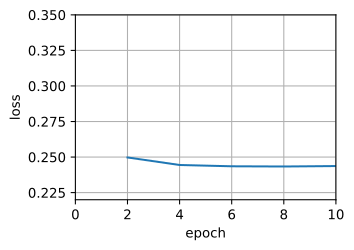
loss: 0.242, 0.056 sec/epoch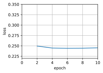
At the opposite extreme, batch size 1 is stochastic gradient descent: 1500 updates per epoch, at a constant (and necessarily small) learning rate. The loss falls quickly at first and then the decline slows. Both procedures process 1500 examples per epoch, but SGD takes more clock time per epoch than gradient descent here: it dispatches 1500 tiny operations where gradient descent dispatches one large operation. The single-example method therefore incurs dispatch overhead at every step.
sgd_res = train_sgd(0.005, 1)loss: 0.243, 0.401 sec/epoch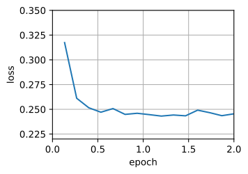
loss: 0.245, 3.175 sec/epoch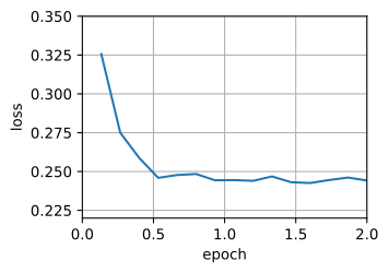
With a batch size of 100 the time per epoch drops below both extremes.
mini1_res = train_sgd(.4, 100)loss: 0.247, 0.016 sec/epoch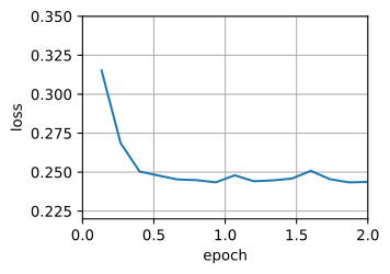
loss: 0.244, 0.309 sec/epoch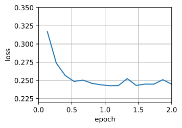
Reducing the batch size to 10 raises the time per epoch again: the work per dispatch is getting too small to run efficiently.
mini2_res = train_sgd(.05, 10)loss: 0.247, 0.055 sec/epoch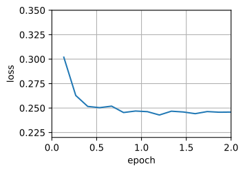
loss: 0.243, 0.628 sec/epoch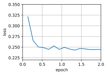
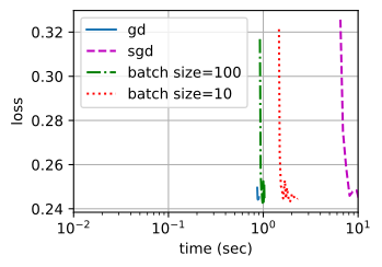
Plotting loss against wall-clock time for all four experiments makes the trade explicit. SGD converges fastest per example processed, yet reaches a given loss slower than gradient descent by the clock, because it computes gradients one example at a time. Minibatch SGD takes both savings at once: batch size 10 beats pure SGD, and batch size 100 beats even gradient descent on runtime.
d2l.set_figsize([6, 3])
d2l.plot(*list(map(list, zip(gd_res, sgd_res, mini1_res, mini2_res))),
         'time (sec)', 'loss', xlim=[1e-2, 10], xscale='log',
         legend=['gd', 'sgd', 'batch size=100', 'batch size=10'])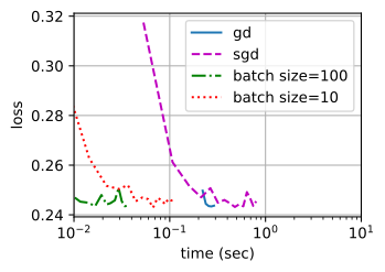
9.4.5 Concise Implementation
Every framework ships these loops behind an optimizer object. Using it makes the training function shorter and less error-prone; we wrap the pattern into a generic function used throughout this chapter.
def train_concise_ch11(trainer_fn, hyperparams, data_iter, num_epochs=4):
    # Initialization
    net = nn.Sequential(nn.Linear(5, 1))
    def init_weights(module):
        if type(module) == nn.Linear:
            torch.nn.init.normal_(module.weight, std=0.01)
    net.apply(init_weights)

    optimizer = trainer_fn(net.parameters(), **hyperparams)
    loss = nn.MSELoss(reduction='none')
    animator = d2l.Animator(xlabel='epoch', ylabel='loss',
                            xlim=[0, num_epochs], ylim=[0.22, 0.35])
    n, timer = 0, d2l.Timer()
    for _ in range(num_epochs):
        for X, y in data_iter:
            optimizer.zero_grad()
            out = net(X)
            y = y.reshape(out.shape)
            l = loss(out, y)
            l.mean().backward()
            optimizer.step()
            n += X.shape[0]
            if n % 200 == 0:
                timer.stop()
                # `MSELoss` computes squared error without the 1/2 factor
                animator.add(n/X.shape[0]/len(data_iter),
                             (d2l.evaluate_loss(net, data_iter, loss) / 2,))
                timer.start()
    print(f'loss: {animator.Y[0][-1]:.3f}, {timer.sum()/num_epochs:.3f} sec/epoch')
def train_concise_ch11(trainer_fn, hyperparams, data_iter, num_epochs=2):
    # Initialization
    net = nnx.Linear(5, 1, rngs=nnx.Rngs(0))
    optimizer = nnx.Optimizer(
        net, trainer_fn(**hyperparams), wrt=nnx.Param)

    loss = lambda pred, y: jnp.mean((pred - y) ** 2) / 2
    animator = d2l.Animator(xlabel='epoch', ylabel='loss',
                            xlim=[0, num_epochs], ylim=[0.22, 0.35])
    n, timer = 0, d2l.Timer()
    # JIT-fuse the per-batch optimizer update so per-step Python overhead
    # stays out of the inner loop.
    @nnx.jit
    def step(model, optimizer, X, y):
        def loss_fn(model):
            out = model(X)
            y_reshaped = y.reshape(out.shape)
            return jnp.mean((out - y_reshaped) ** 2) / 2
        l, grads = nnx.value_and_grad(loss_fn)(model)
        optimizer.update(model, grads)
        return l

    # Pre-stack the full dataset on device so the periodic full-loss
    # evaluation is a single compiled call.
    eval_batches = [(jnp.array(X), jnp.array(y)) for X, y in data_iter]
    Xs = jnp.concatenate([X for X, _ in eval_batches], axis=0)
    ys = jnp.concatenate([y for _, y in eval_batches], axis=0)
    @nnx.jit
    def full_eval(model):
        out = model(Xs)
        y_r = ys.reshape(out.shape)
        return jnp.mean((out - y_r) ** 2) / 2
    for _ in range(num_epochs):
        for X, y in data_iter:
            X, y = jnp.array(X), jnp.array(y)
            step(net, optimizer, X, y)
            n += X.shape[0]
            if n % 200 == 0:
                timer.stop()
                animator.add(n/X.shape[0]/len(data_iter),
                             (float(full_eval(net)),))
                timer.start()
    print(f'loss: {animator.Y[0][-1]:.3f}, {timer.sum()/num_epochs:.3f} sec/epoch')
Repeating the batch-size-10 experiment through the framework optimizer shows the same behavior.
data_iter, _ = get_data_ch11(10)
trainer = torch.optim.SGD
train_concise_ch11(trainer, {'lr': 0.01}, data_iter)
loss: 0.243, 0.058 sec/epoch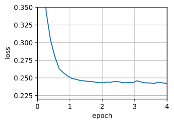
data_iter, _ = get_data_ch11(10)
trainer = optax.sgd
train_concise_ch11(trainer, {'learning_rate': 0.05}, data_iter)
loss: 0.243, 0.350 sec/epoch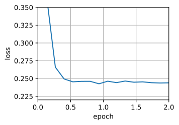
9.4.6 Summary
Minibatches are cheap for mechanical reasons: a batched operation shares one round of dispatch overhead and one pass over the weights across \(b\) examples, and blocked computation keeps data in cache, where the same processor runs orders of magnitude faster than when it waits on main memory. Combined with the \(1/b\) variance reduction measured in Section 9.3, this is why minibatch SGD reaches a target loss sooner than either extreme in this section’s timing comparison. Choosing \(b\) to fill the device without exhausting its memory captures most of the benefit; Section 9.10 then asks how far the statistics allow batch size to grow before the returns vanish, a limit known as the critical batch size.
9.4.7 Exercises
- [code] Batch size and learning rate together. ●
train_sgdtrains the linear model at a chosen batch size and learning rate and returns the cumulative wall-clock times and the recorded losses. Fix \(\eta = 0.05\) at \(b = 10\) and derive the learning rate for each \(b \in \{1, 10, 100, 1000\}\) by two rules, \(\eta \propto \sqrt{b}\) and \(\eta \propto b\).Train each configuration for two epochs. Report the time per epoch and the final loss of each run, and name the runs that diverge.
The training loss is a quadratic in the weights and the bias. Its Hessian is
\[\mathbf{H} = \frac{1}{n} \sum_{i=1}^{n} \tilde{\mathbf{x}}_i \tilde{\mathbf{x}}_i^\top, \tag{9.4.3}\]
where \(\tilde{\mathbf{x}}_i\) appends a constant \(1\) to the features of example \(i\) and \(n = 1500\). Compute the largest eigenvalue \(L\) of \(\mathbf{H}\) from the whitened data that
get_data_ch11loads. Use the condition \(0 < \eta < 2/L\) of Section 9.2 to explain which runs diverge.At \(b = 1\), which rule reaches the lower final loss? Explain the ordering with Equation 9.3.5.
- [code] Block width and throughput. The blocked computation in Section 9.4.2 multiplies 64 columns of \(\mathbf{C}\) at a time.
- Vary the block width \(w\) over \(\{1, 4, 16, 64, 256\}\). Time each variant with
timerafter one untimed warm-up run, and report its throughput in gigaflops. Then divide each time by the number of calls, \(256/w\). Use the time per call to decide, for each width, whether dispatch overhead or arithmetic dominates. - Repeat the column-wise and one-call computations of Section 9.4.1 and the blocked computation with \(4096 \times 4096\) matrices on a GPU, waiting for the device to finish before each
timer.stop(). Which ratios between the variants change, and what does the change say about dispatch overhead relative to arithmetic?
- Vary the block width \(w\) over \(\{1, 4, 16, 64, 256\}\). Time each variant with
- Duplicated data. Suppose every example in the training set is silently duplicated, so that the dataset doubles in size while its empirical distribution is unchanged. For SGD with \(b = 1\), for minibatch SGD at a fixed \(b\), and for full-batch gradient descent, state whether the cost per step, the number of steps to reach a given loss, and the variance of the gradient estimate change, and explain each answer.
- [code] Gradient accumulation. Implement gradient accumulation on top of
train_ch11: sum the gradients of \(k\) consecutive minibatches of size \(b\) and update once with their average.- Take \(b = 10\), \(k = 10\) and the learning rate \(0.05\). Set the same random seed before this run and before a run with batch size \(kb = 100\) at the same learning rate, so that both draw the same initial weights and the same example order. Plot both loss trajectories against the number of examples processed and report the largest difference between them.
- Remove the division by \(k\), so that the update uses the sum of the \(k\) gradients. Which learning rate of the batch-size-100 run does the accumulated run now reproduce?
- Compare the two runs of (a) against wall-clock time. Which costs more per example, and where in the code does the difference arise?