%matplotlib inline
from d2l import torch as d2l
import math
import torch
from torch.nn import functional as F9.7 AdamW
Adam is commonly used with decoupled weight decay, producing AdamW: Adam with a separate shrinkage update applied to selected parameter groups. The coefficient depends on the model, schedule, training horizon, and parameter group; later examples report values used in specific language-model recipes. This section explains the W. Back in Section 2.7 we saw that adding an \(\ell_2\) penalty to the loss and shrinking the weights by a fixed factor each step are the same operation under stochastic gradient descent. Under Adam, however, the adaptive preconditioner changes the penalty coordinate by coordinate, so the two operations are no longer equivalent. The decoupled update of Loshchilov and Hutter (2019) restores direct control over the shrinkage. This section derives and measures the difference.
We first derive the loss-penalty and decoupled updates, then implement AdamW and compare both forms on the language model of Section 9.6.2. The final sections discuss the effect of weight decay in large-scale training, the parameters commonly exempted from it, and the memory required for optimizer state.
%matplotlib inline
from d2l import jax as d2l
from flax import nnx
import jax
from jax import numpy as jnp
import math
import optax
9.7.1 The Penalty Meets the Preconditioner
Add the penalty \(\frac{\lambda}{2}\|\mathbf{x}\|^2\) to the loss and the gradient becomes \(\mathbf{g}_t + \lambda \mathbf{x}_t\). Under SGD the two implementations of weight decay coincide, as we saw in Section 2.7:
\[ \mathbf{x}_{t+1} = \mathbf{x}_t - \eta\,(\mathbf{g}_t + \lambda \mathbf{x}_t) = (1 - \eta\lambda)\,\mathbf{x}_t - \eta\,\mathbf{g}_t. \tag{9.7.1}\]
Penalizing the loss is shrinking the weights, by the uniform factor \(1 - \eta\lambda\). Now feed the same penalized gradient through Adam’s update Equation 9.6.4. The moments are built from the penalized gradient, so the penalty also passes through the adaptive preconditioner. The following display is schematic: treating \(\sqrt{\hat{\mathbf{v}}_t}\) as a common preconditioner for loss term and penalty alike (both moments are in fact built from the penalized gradient), the shrinkage applied to coordinate \(i\) is no longer uniform:
\[ \underbrace{\frac{\eta\,\lambda}{\sqrt{\hat{v}_{t,i}} + \epsilon}\; x_{t,i}}_{\textrm{$\ell_2$ penalty through Adam}} \qquad \textrm{versus} \qquad \underbrace{\eta\,\lambda\; x_{t,i}\vphantom{\frac{\eta}{\sqrt{\hat{v}_{t,i}}}}}_{\textrm{weight decay}}. \tag{9.7.2}\]
The regularization strength is now rescaled per coordinate by the same preconditioner that rescales the loss gradient, and backwards: a parameter with a large gradient history (large \(\hat{v}_i\)) is barely decayed at all, while a parameter with a small gradient history receives much stronger effective decay. Whatever \(\lambda\) you chose, Adam changes its effective value by coordinate and over time. The appendix works this out exactly and isolates it in a two-coordinate experiment where the same \(\lambda\) produces effective decay rates \(100\times\) apart (Section 26.2.3).
AdamW restores the SGD semantics by decoupling: the loss gradient goes through the preconditioner and the decay does not,
\[ \mathbf{x}_{t+1} = (1 - \eta\lambda)\,\mathbf{x}_t - \eta\, \frac{\hat{\mathbf{m}}_t}{\sqrt{\hat{\mathbf{v}}_t} + \epsilon}, \tag{9.7.3}\]
with \(\hat{\mathbf{m}}_t\) and \(\hat{\mathbf{v}}_t\) computed from the plain gradient \(\mathbf{g}_t\) as in Equation 9.6.3. This is verbatim the shrink factor of Equation 9.7.1, applied uniformly. When the learning rate follows a schedule \(\eta_t\), the decay follows the same schedule: Loshchilov and Hutter (2019) scale the decay term by the schedule multiplier so that regularization does not outlive learning, and the implementations in PyTorch and Optax fold the entire learning rate into the decay, which is the convention we use throughout.
9.7.2 AdamW from Scratch
The implementation is Adam from Section 9.6 plus one term in the update. We keep the same state layout, two buffers per parameter, and add the decay coefficient to the hyperparameter dictionary.
def init_adamw_states(feature_dim):
    m_w, m_b = d2l.zeros((feature_dim, 1)), d2l.zeros(1)
    v_w, v_b = d2l.zeros((feature_dim, 1)), d2l.zeros(1)
    return ((m_w, v_w), (m_b, v_b))

def adamw(params, states, hyperparams):
    beta1, beta2, eps = 0.9, 0.999, 1e-6
    for p, (m, v) in zip(params, states):
        with torch.no_grad():
            m[:] = beta1 * m + (1 - beta1) * p.grad
            v[:] = beta2 * v + (1 - beta2) * torch.square(p.grad)
            m_hat = m / (1 - beta1 ** hyperparams['t'])
            v_hat = v / (1 - beta2 ** hyperparams['t'])
            p[:] -= hyperparams['lr'] * (m_hat / (torch.sqrt(v_hat) + eps)
                                         + hyperparams['wd'] * p)
        p.grad.zero_()
    hyperparams['t'] += 1
def init_adamw_states(feature_dim):
m_w, m_b = jnp.zeros((feature_dim, 1)), jnp.zeros(1)
v_w, v_b = jnp.zeros((feature_dim, 1)), jnp.zeros(1)
return [(m_w, v_w), (m_b, v_b)]
def adamw(params, grads, states, hyperparams):
beta1, beta2, eps = 0.9, 0.999, 1e-6
for i, (p, (m, v), g) in enumerate(zip(params, states, grads)):
m = beta1 * m + (1 - beta1) * g
v = beta2 * v + (1 - beta2) * jnp.square(g)
m_hat = m / (1 - beta1 ** hyperparams['t'])
v_hat = v / (1 - beta2 ** hyperparams['t'])
params[i] = p - hyperparams['lr'] * (
m_hat / (jnp.sqrt(v_hat) + eps) + hyperparams['wd'] * p)
states[i] = (m, v)
hyperparams['t'] += 1
return params[0], params[1]On the airfoil harness of Section 9.4 it behaves like Adam with a mild pull toward small weights; on a well-conditioned regression problem there is little for the decay to do, and that is the point: decoupled decay is a knob you can leave gently on without disturbing the optimizer.
data_iter, feature_dim = d2l.get_data_ch11(batch_size=10)
d2l.train_ch11(adamw, init_adamw_states(feature_dim),
{'lr': 0.01, 'wd': 0.01, 't': 1}, data_iter, feature_dim);loss: 0.246, 0.129 sec/epoch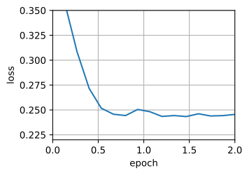
loss: 0.244, 1.792 sec/epoch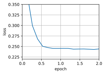
The framework implementations follow Equation 9.7.3 up to small conventions that differ by framework and version — \(\epsilon\) placement, optional flags, and whether the decay is scaled by the learning rate.
trainer = torch.optim.AdamW
d2l.train_concise_ch11(trainer, {'lr': 0.01, 'weight_decay': 0.01},
                       data_iter)
loss: 0.244, 0.102 sec/epoch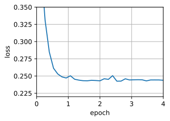
trainer = optax.adamw
d2l.train_concise_ch11(trainer,
                       {'learning_rate': 0.01, 'weight_decay': 0.01},
                       data_iter)
loss: 0.243, 0.406 sec/epoch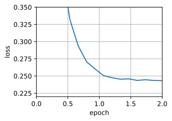
A note on defaults before we move on. AdamW inherits Adam’s \((\beta_1, \beta_2) = (0.9, 0.999)\), but large language models are commonly trained with \(\beta_2 = 0.95\), a convention set by GPT-3 (Brown et al. 2020) and kept by many open recipes since, including OLMo 2 (Team OLMo et al. 2025) (not all: PaLM did not (Chowdhery et al. 2022)). The shorter second-moment window (about twenty steps instead of a thousand) makes the scale estimate track heavy-tailed gradient noise faster, at some cost in smoothing; we return to its effect in Section 9.12. One property that has changed into practice is Adam’s original claim that the method is robust to its hyperparameters; both \(\eta\) and \(\lambda\) still need to be chosen, and the next experiment is about whether they can at least be chosen independently.
9.7.3 Decoupling, Demonstrated
We return to the testbed of Section 9.6.2: TinyLM on the character-level Time Machine, with the same helpers for the final loss and a smoothed curve.
data = d2l.TimeMachine(batch_size=64, num_steps=64, tokenization='char',
                       num_train=100000)

def final_loss(losses, k=100):
    v = sum(losses[-k:]) / k
    return v if math.isfinite(v) else float('inf')

def smooth(losses, k=25):
    return [sum(losses[i:i + k]) / k
            for i in range(0, len(losses) - k + 1, k)]
Weight decay concerns generalization, so we also need a metric that the training loss cannot see: the mean cross-entropy on held-out text.
def val_loss(model, data):
    device = d2l.try_gpu()
    model.eval()
    total, count = 0.0, 0
    with torch.no_grad():
        for X, Y in data.val_dataloader():
            X, Y = X.to(device), Y.to(device)
            logits = model(X)
            total += float(F.cross_entropy(
                logits.reshape(-1, logits.shape[-1]), Y.reshape(-1),
                reduction='sum'))
            count += Y.numel()
    return total / count
@nnx.jit
def eval_step(model, X, Y):
logits = model(X)
return optax.softmax_cross_entropy_with_integer_labels(
logits.reshape(-1, logits.shape[-1]), Y.reshape(-1)).sum()
def val_loss(model, data):
total, count = 0.0, 0
for X, Y in data.val_dataloader():
total += float(eval_step(model, jnp.asarray(X), jnp.asarray(Y)))
count += Y.reshape(-1).shape[0]
return total / count9.7.3.1 Interaction between Learning Rate and Decay
First, the size of the problem. We train TinyLM twice, each framework at its own tuned learning rate from Section 9.6, with the standard \(\lambda = 0.1\), once as an \(\ell_2\) penalty inside Adam’s gradient, and once decoupled as AdamW. In PyTorch the coupled version is what Adam’s weight_decay argument does; in Optax we build it by adding the decay to the gradient before it enters adam. The number \(\lambda\) is nominally identical in both runs.
curves = {}
for name, opt_cls in [('Adam + $\\ell_2$', torch.optim.Adam),
                      ('AdamW', torch.optim.AdamW)]:
    torch.manual_seed(0)
    model = d2l.TinyLM(len(data.vocab))
    optimizer = opt_cls(model.parameters(), lr=0.003, weight_decay=0.1)
    curves[name] = d2l.train_lm(model, data, optimizer, num_steps=1000)
d2l.plot(list(range(0, 1000, 25)), [smooth(c) for c in curves.values()],
         'step', 'training loss', legend=list(curves))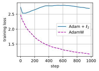
def coupled(lr, wd):
    return optax.chain(optax.add_decayed_weights(wd), optax.adam(lr))

curves = {}
for name, tx in [('Adam + $\\ell_2$', coupled(0.001, 0.1)),
                 ('AdamW', optax.adamw(0.001, weight_decay=0.1))]:
    model = d2l.TinyLM(len(data.vocab), rngs=nnx.Rngs(0))
    optimizer = nnx.Optimizer(model, tx, wrt=nnx.Param)
    curves[name] = d2l.train_lm(model, data, optimizer, num_steps=1000)
d2l.plot(list(range(0, 1000, 25)), [smooth(c) for c in curves.values()],
         'step', 'training loss', legend=list(curves))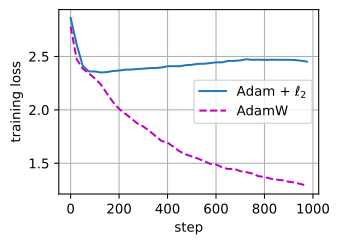
The decoupled run reaches nearly the same training loss as the no-decay baseline. The coupled run remains more than a full nat higher, only slightly below its starting loss. The mechanism is Equation 9.7.2 read as an amplifier: once training makes progress the loss gradients shrink, \(\sqrt{\hat{\mathbf{v}}}\) shrinks with them, and the penalty, divided by that small number, comes back amplified by orders of magnitude. Worse, once \(\lambda \mathbf{x}\) dominates the gradient, Adam normalizes it like any other gradient: every coordinate then shrinks at a rate near \(\eta\) regardless of \(\lambda\), so past this point the dial no longer responds. Under coupled decay, \(\lambda = 0.1\) does not specify one uniform amount of regularization. The preconditioner changes its effect by coordinate, step, and problem.
9.7.3.2 A Grid, Twice
The claim worth testing is not that coupled decay is too strong; you could always compensate with a smaller \(\lambda\). It is that the compensation depends on the learning rate, so the two knobs must be tuned jointly, whereas decoupling lets them be tuned separately. So we run the same experiment twice: a \(3 \times 3\) grid of learning rate against weight decay, once coupled, once decoupled, scored by held-out loss.
To make the effect of decay measurable, we use a setting with repeated training data and visible overfitting: a training slice of 8,000 windows that the model revisits about six times in 800 steps. (On the full corpus the model barely completes one pass, and in our runs two orders of magnitude of \(\lambda\) move the held-out loss by a few hundredths of a nat: at this scale, weight decay is a knob for data you repeat. The later discussion considers decay in genuinely one-pass training at much larger scale.) Each arm receives a suitable \(\lambda\) range. The resulting scales already differ substantially: the coupled arm needs values two to three orders of magnitude smaller to land anywhere near its sweet spot.
small = d2l.TimeMachine(batch_size=64, num_steps=64, tokenization='char',
num_train=8000, num_val=2000)lrs = [1e-3, 3e-3, 1e-2]
wds_coupled, wds_decoupled = [3e-4, 1e-3, 3e-3], [1, 3, 10]
def sweep(make_optimizer, wds, num_steps=800):
tbl = []
for lr in lrs:
row = []
for wd in wds:
torch.manual_seed(0)
model = d2l.TinyLM(len(small.vocab))
d2l.train_lm(model, small, make_optimizer(model, lr, wd),
num_steps)
row.append(val_loss(model, small))
tbl.append(row)
print(' '.join(f'{v:.2f}' for v in row))
return tbl
coupled_tbl = sweep(lambda model, lr, wd: torch.optim.Adam(
model.parameters(), lr, weight_decay=wd), wds_coupled)3.62 2.11 2.33
4.10 2.70 2.34
4.09 2.37 2.34lrs = [3e-4, 1e-3, 3e-3]
wds_coupled, wds_decoupled = [3e-3, 1e-2, 3e-2], [1, 3, 10]
def sweep(make_tx, wds, num_steps=800):
tbl = []
for lr in lrs:
row = []
for wd in wds:
model = d2l.TinyLM(len(small.vocab), rngs=nnx.Rngs(0))
optimizer = nnx.Optimizer(model, make_tx(lr, wd),
wrt=nnx.Param)
d2l.train_lm(model, small, optimizer, num_steps)
row.append(val_loss(model, small))
tbl.append(row)
print(' '.join(f'{v:.2f}' for v in row))
return tbl
coupled_tbl = sweep(coupled, wds_coupled)2.65 2.26 2.18
3.15 2.22 2.37
2.72 2.33 2.39decoupled_tbl = sweep(lambda model, lr, wd: torch.optim.AdamW(
model.parameters(), lr, weight_decay=wd), wds_decoupled)3.02 2.11 2.56
3.19 2.08 2.49
2.98 2.31 2.57decoupled_tbl = sweep(lambda lr, wd: optax.adamw(lr, weight_decay=wd),
wds_decoupled)2.66 2.29 2.44
3.18 2.31 2.58
3.04 2.25 2.52def show_grids(tables, wd_axes, titles):
fig, axes = d2l.plt.subplots(1, 2, figsize=(7, 3), sharey=True)
lo = min(v for tbl in tables for row in tbl for v in row)
hi = max(v for tbl in tables for row in tbl for v in row)
for ax, tbl, wds, title in zip(axes, tables, wd_axes, titles):
ax.imshow(tbl, cmap='viridis', vmin=lo, vmax=hi)
for i, row in enumerate(tbl):
best = min(range(len(row)), key=lambda j: row[j])
for j, v in enumerate(row):
ax.text(j, i, f'{v:.2f}', ha='center', va='center',
color='black' if (v - lo) / (hi - lo) > 0.5
else 'white',
fontweight='bold' if j == best else 'normal')
i, j = min(((i, j) for i, row in enumerate(tbl)
for j in range(len(row))),
key=lambda ij: tbl[ij[0]][ij[1]])
ax.add_patch(d2l.plt.Rectangle((j - 0.5, i - 0.5), 1, 1, fill=False,
edgecolor='red', lw=2))
ax.set_xticks(range(len(wds)), [f'{wd:g}' for wd in wds])
ax.set_yticks(range(len(lrs)), [f'{lr:g}' for lr in lrs])
ax.set_xlabel('weight decay $\\lambda$')
ax.set_title(title)
axes[0].set_ylabel('learning rate $\\eta$')
show_grids([coupled_tbl, decoupled_tbl],
[wds_coupled, wds_decoupled],
['Adam + $\\ell_2$', 'AdamW'])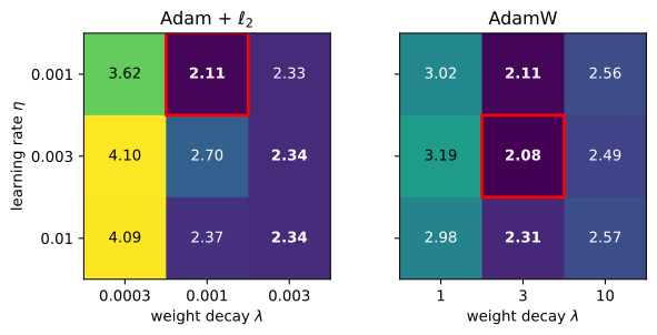
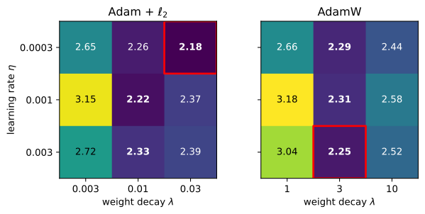
Read each heatmap row by row; the two panels share one color scale, the best \(\lambda\) in each row is set in bold, and each panel’s best cell is boxed in red. In the AdamW grid the bold entries line up in a single column: the best weight decay is the same at every learning rate in the grid, and in this single-seed run the same column wins in both frameworks, despite the frameworks’ different initializations. In the coupled grid the bold entries wander: change \(\eta\) and the tuned \(\lambda\) is no longer optimal, exactly the joint-tuning burden that Loshchilov and Hutter (2019) documented on image classifiers, where the good region of the coupled \((\eta, \lambda)\) plane is a diagonal band and the decoupled one is axis-aligned. Note what decoupling does not change at this scale: after tuning both arms fully, their best held-out losses are close. The practical difference is that one of the two searches was a line search and the other genuinely needed the grid.
9.7.3.3 What Weight Decay Is Actually Doing
Section 2.7 introduced weight decay as a regularizer, a Gaussian prior shrinking the model toward simple functions, and our overfitting experiment above used it that way. Modern large-scale practice mostly does not. A language model trained for a single epoch on non-repeated data has little classical overfitting to fight, yet \(\lambda = 0.1\) remains in every frontier recipe. What is it doing there?
Careful ablations (D’Angelo et al. 2024; Kosson et al. 2024) have assembled the current understanding: weight decay at scale is a training-dynamics control, not an explicit regularizer. The mechanism runs through the weight norms. A weight matrix whose output is consumed only through a normalization layer is scale-invariant: rescaling the matrix leaves the network’s function unchanged, because the norm discards the scale, so only the direction of the weight vector matters and the effective step size of an update is roughly the update divided by the weight norm. This is exact for a weight immediately followed by a normalization layer; in a pre-LN residual transformer it holds only approximately, since the residual stream carries each block’s output around the next norm rather than through it. It still describes enough of the parameters to drive the dynamics below. Gradient noise pushes weight norms up; decay pulls them down; the two settle into an equilibrium, a steady state that Kosson et al. (2024) describe as rotational, in which each weight vector turns by a roughly constant angle per step. Through this equilibrium \(\lambda\) sets the effective learning rate, and sets it uniformly across layers. That is a large part of why decayed LLM runs reach lower training loss rather than trading training loss for validation loss, the signature D’Angelo et al. (2024) document. Decay performs a second, mundane service too: it keeps parameters small enough that bfloat16 training does not wander into divergence.
Two consequences carry forward. First, since the decay term is multiplied by the schedule, \(\eta\) and \(\lambda\) act on the equilibrium through their product, and what the product controls is a timescale: an AdamW iterate is approximately an average of its recent updates over a horizon of \(1/(\eta\lambda)\) steps. In epoch units the horizon is \(\tau = B/(\eta \lambda D)\) for batch size \(B\) and dataset size \(D\), and recent scaling studies find that \(\tau\) is the quantity to hold roughly steady, so that \(\lambda\) is co-varied with batch and dataset size rather than re-tuned (Bergsma et al. 2025). Second, none of this mechanism applies to parameters that are not followed by normalization, which is why the next section can give a sharper answer than “all of them” to the question of which parameters to decay.
9.7.4 What Not to Decay
The parameter census of Section 9.6.2 sorted TinyLM into three populations: embeddings, two-dimensional matrices, and one-dimensional vectors, the LayerNorm scales and biases. Standard practice decays only the matrices.
The reasons differ by population. LayerNorm scales and biases are few, and they set the model’s normalization scales directly, so shrinking them toward zero directly disrupts those normalization scales; they are left alone, as biases were already in Section 2.7. Embedding rows are sparse: a row receives a gradient only when its token occurs, but decay is applied every step, so rare rows are all decay and no signal. OLMo 2 traced a training instability to exactly this: decay ground the embedding norms down until the \(1/\|\mathbf{x}\|\) factor in LayerNorm’s gradient blew the early layers up. The fix was to turn decay off for embeddings and let their norms settle (Team OLMo et al. 2025).
The implementation pattern is two parameter groups, and the census already computed the split. In PyTorch, torch.optim.AdamW takes a list of groups with per-group settings; in Optax, optax.adamw takes a mask over the parameter tree. The same split returns in Section 9.9, where the matrices receive a different optimizer rather than only a different decay setting.
torch.manual_seed(0)
model = d2l.TinyLM(len(data.vocab))
decay = [p for name, p in model.named_parameters()
         if p.ndim == 2 and 'emb' not in name]
no_decay = [p for name, p in model.named_parameters()
            if p.ndim != 2 or 'emb' in name]
optimizer = torch.optim.AdamW([
    {'params': decay, 'weight_decay': 0.1},
    {'params': no_decay, 'weight_decay': 0.0}], lr=0.003)
n_decay = sum(p.numel() for p in decay)
n = n_decay + sum(p.numel() for p in no_decay)
print(f'decayed: {n_decay} of {n} parameters')
decayed: 396800 of 412188 parametersmodel = d2l.TinyLM(len(data.vocab), rngs=nnx.Rngs(0))
def decay_mask(params):
return jax.tree_util.tree_map_with_path(
lambda path, p: p.ndim == 2 and 'emb' not in str(path), params)
optimizer = nnx.Optimizer(
model, optax.adamw(0.001, weight_decay=0.1, mask=decay_mask),
wrt=nnx.Param)
params = nnx.state(model, nnx.Param)
n_decay = sum(int(p.size) for p, m in zip(
jax.tree.leaves(params), jax.tree.leaves(decay_mask(params))) if m)
n = sum(int(p.size) for p in jax.tree.leaves(params))
print(f'decayed: {n_decay} of {n} parameters')decayed: 396800 of 412188 parametersAbout 96% of the parameters are decayed; normalization parameters, biases, and embeddings are exempt. Trained on the full corpus, the two-group configuration matches the tuned Adam run of Section 9.6:
losses = d2l.train_lm(model, data, optimizer, num_steps=2000)
d2l.plot(list(range(0, 2000, 25)), [smooth(losses)],
         'step', 'training loss')
print(f'perplexity per character: {math.exp(final_loss(losses)):.2f}')perplexity per character: 2.62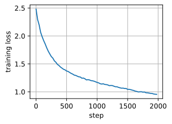
perplexity per character: 2.76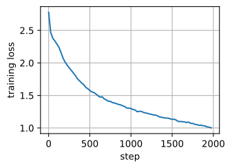
This is the modern default configuration in full: AdamW, decay on the matrices only, \(\lambda\) chosen jointly with the schedule. What remains is to ask what it costs.
9.7.5 Memory Required for Optimizer State
Adam and AdamW carry two extra numbers per parameter, \(m\) and \(v\). At this chapter’s scale that is invisible; at language-model scale it decides what fits on a device, so we do the arithmetic once with real numbers, using the parameter total \(n\) computed above.
In full fp32 training, a parameter costs 4 bytes each for the weight, the gradient, \(m\), and \(v\): 16 bytes per parameter, three quarters of it the optimizer’s. Mixed-precision training in bf16 does not make this smaller, it makes it larger: the weights and gradients used in the forward and backward pass drop to 2 bytes, but stable training keeps an fp32 master copy of the weights alongside the optimizer state, and usually an fp32 accumulator for gradients as well (Section 30.6).
setups = {'fp32 weights, grads, m, v': (4, 4, 8),
          'bf16 weights + grads, fp32 master, m, v': (2, 2, 12),
          'the same + fp32 gradient accumulator': (2, 6, 12)}
print(f'{"":<42}{"B/param":>8}{"TinyLM":>10}{"7B model":>10}')
for name, (w, g, s) in setups.items():
    per = w + g + s
    print(f'{name:<42}{per:>8}{n * per / 1e6:>8.1f}MB'
          f'{7e9 * per / 1e9:>8.0f}GB')
B/param TinyLM 7B model
fp32 weights, grads, m, v 16 6.6MB 112GB
bf16 weights + grads, fp32 master, m, v 16 6.6MB 112GB
the same + fp32 gradient accumulator 20 8.2MB 140GBFor TinyLM the total is a few megabytes. Scale the identical arithmetic to a 7-billion-parameter model and the common bf16 pattern costs about 140 GB before a single activation is stored, more than any single 80-GB accelerator holds. Of the 20 bytes per parameter, 12 belong to the optimizer: the fp32 master, \(m\), and \(v\). That ratio is why optimizer state is the first target when memory runs out. Adafactor factors \(v\) for each matrix into a row and a column sum, replacing \(mn\) numbers by \(m + n\) (Shazeer and Stern 2018); 8-bit optimizers store \(m\) and \(v\) block-quantized at one byte each (Dettmers et al. 2022). The other lever is not shrinking the state but not replicating it: ZeRO-style sharding spreads the 20 bytes across the data-parallel group (Rajbhandari et al. 2020), a systems technique discussed in Chapter 13 and Section 30.6.
9.7.6 Summary
Under SGD, an \(\ell_2\) penalty in the loss and a per-step shrinkage of the weights are the same thing; under Adam they are not, because the penalty’s gradient is divided by \(\sqrt{\hat{\mathbf{v}}}\) along with the loss gradient. This rescales regularization separately for each coordinate and reverses the intended dependence on gradient scale. AdamW applies the decay outside the preconditioner, restoring one \(\lambda\) with one meaning. Decoupling does not so much improve the best attainable loss as make it findable: in our grid the best \(\lambda\) stopped depending on the learning rate. At scale, weight decay is less a regularizer than a training-dynamics control that sets the effective learning rate through an equilibrium of noise against decay, on a timescale set by the product \(\eta\lambda\). Decay the matrices; exempt embeddings, norms, and biases. With the standard mixed-precision pattern, an AdamW parameter costs about 20 bytes, 12 of them optimizer state.
9.7.7 Exercises
- [code] Saturation of coupled decay. The experiment of Section 26.2.3 starts two parameters at \(x_i = 1\) and gives them pure-noise loss gradients \(g_i \sim \mathcal{N}(0, \sigma_i^2)\) with \(\sigma = (10, 0.1)\). At \(\eta = 10^{-3}\) and \(\lambda = 0.1\), Adam with an \(\ell_2\) penalty decays them at the rates \(\eta\lambda/\sigma_i\) that Equation 9.7.2 predicts.
- In the opposite limit \(\sigma_i = 0\), the penalized gradient is \(\lambda x_{t,i}\) alone. Show that for \(\epsilon = 0\) the trajectory of \(x_{t,i}\) under Adam with an \(\ell_2\) penalty does not depend on \(\lambda > 0\).
- Extend the experiment to \(\sigma_i \in \{10, 1, 0.1, 0.01, 0.001\}\) at \(\eta = 10^{-3}\) and record \(|x_i|\) after 1,000 steps of Adam with an \(\ell_2\) penalty for each \(\lambda \in \{0.1, 1, 10\}\). Which coordinates no longer respond to \(\lambda\), and how does the transition between the two regimes depend on \(\sigma_i\) and \(\lambda\)?
- [code] Momentum and the penalty. ● Under SGD with momentum, an \(\ell_2\) penalty adds \(\lambda \mathbf{x}_{t-1}\) to the gradient \(\mathbf{g}_t\) in the velocity of Equation 9.5.2. Decoupled decay leaves the velocity alone and shrinks the weights directly: \[\mathbf{v}_t = \beta \mathbf{v}_{t-1} + \mathbf{g}_t, \qquad
\mathbf{x}_t = (1 - \eta\lambda)\,\mathbf{x}_{t-1} - \eta\,\mathbf{v}_t.\]
- Unroll the coupled velocity and compute the total shrinkage that the penalty term \(\lambda \mathbf{x}_{t-1}\) of one step applies to the weights over all later steps. Are the two updates equivalent at the same \(\lambda\)? Does their difference depend on the coordinate, as it does under Adam?
- Modify
sgd_momentumof Section 9.5 to implement both updates, and train each withd2l.train_ch11on the airfoil data atlr=0.02andmomentum=0.9. Run the coupled update at \(\lambda = 1\) and the decoupled update at \(\lambda \in \{1, 3, 10, 30\}\). Which decoupled coefficient comes closest to the coupled run’s final training loss, and how does it compare with your answer to the first part?
- [code] The fixed-product ridge. ● Both library implementations used in this section multiply the decay by the full learning rate, so the per-step shrinkage is \(s = \eta\lambda\). Section 9.7.3.3 argues that at scale \(\eta\) and \(\lambda\) act through this product, which sets an averaging horizon of \(1/s\) steps. Loshchilov and Hutter (2019) instead scale the decay by the schedule multiplier only, so that under a constant schedule their decay coefficient is \(s\) itself.
- Each column of a grid can fix \(s\) instead of \(\lambda\). Use
decoupled_tblto predict where the best entry of each row falls on the shrinkage axis[1e-3, 3e-3, 1e-2, 3e-2]. Then rerun the decoupled grid of Section 9.7.3.2 withsweepon this axis, passing the decay coefficient to the optimizer aswd / lr. Does the best column stay put? - How constant is the held-out loss down the column \(s = 3 \times 10^{-3}\)? Reconcile the answer with the argument of Section 9.7.3.3, and state which quantity, \(\lambda\) or \(s\), the decay axis of a grid should carry when the learning rate is retuned in this setting.
- Each column of a grid can fix \(s\) instead of \(\lambda\). Use
- [code] Rotational equilibrium. ● Following Kosson et al. (2024), let \(\mathbf{x} \in \mathbb{R}^d\) be a scale-invariant weight vector in the sense of Section 9.7.3.3, trained by AdamW with \(\beta_1 = 0\): \[\mathbf{x}_{t+1} = (1 - \eta\lambda)\,\mathbf{x}_t - \eta\,\mathbf{u}_t,
\qquad \mathbf{u}_t = \frac{\mathbf{g}_t}{\sqrt{\hat{\mathbf{v}}_t} + \epsilon}. \tag{9.7.4}\]
- Show that the loss gradient of a scale-invariant weight vector is orthogonal to \(\mathbf{x}\). Assume from here on that \(\mathbf{u}_t\) is orthogonal to \(\mathbf{x}_t\) as well and that \(\|\mathbf{u}_t\|^2 \approx d\). Derive, to first order in \(\eta\lambda\), the equilibrium norm at which decay balances the growth caused by the updates.
- Derive the angle through which \(\mathbf{x}\) turns per step at equilibrium. How do the equilibrium norm and the angle each depend on \(\eta\) and \(\lambda\)? Relate the result to the claim of Section 9.7.3.3 that \(\eta\) and \(\lambda\) act through their product.
- Check both predictions in numpy with \(d = 1{,}000\) over 20,000 steps from a random unit vector, using pure-noise gradients projected orthogonal to \(\mathbf{x}_t\), at \((\eta, \lambda) \in \{(10^{-3}, 0.1), (3 \times 10^{-3}, 0.1), (10^{-3}, 0.3)\}\).
- [code] Testing the exemptions. Section 9.7.4 attributes OLMo 2’s embedding instability to decay shrinking embedding rows until the \(1/\|\mathbf{x}\|\) factor in the LayerNorm gradient grows large.
- Rerun the two-group configuration with decay applied to every parameter and, in both runs, track the norm of the rarest and of the most frequent token’s embedding row over 2,000 steps.
- Do the two loss curves differ within this budget? Estimate, from the rate at which the rare row shrinks, how many steps the all-decayed run would need before that row’s norm falls by a factor of ten.
- Activations and optimizer state. Extend the accounting of Section 9.7.5 beyond the
setupstable.- For
TinyLMwith batch size \(B\) and sequence length \(T\), estimate the bf16 activation memory that must be stored for the backward pass (per block: the two normalization outputs, the attention inputs and outputs, and the MLP hidden layer). At what batch size do activations overtake the optimizer state? - Count the floating-point operations of one
adamwupdate per parameter and compare them with the roughly \(6BT\) operations per parameter of a forward and backward pass over one batch. At which batch size would the optimizer step cost one percent of a training step?
- For