%matplotlib inline
from d2l import torch as d2l
import torch
from torch import nn11.5 Vision Transformer
The transformer models considered so far operate on text, but their blocks process vectors without assuming that they represent words. This section applies the same blocks to vectors obtained from image patches.
Convolutional networks encode locality and translation equivariance (Section 6.1), whereas a plain transformer block does not. Early attention-based vision models retained local structure: Ramachandran et al. (2019) used local self-attention, and Cordonnier et al. (2020) analyzed conditions under which self-attention can express convolutional operations. The vision transformer (ViT) of Dosovitskiy et al. (2021) divides an image into \(16 \times 16\) patches, embeds each patch as a token, and applies an unmodified transformer encoder to the resulting sequence. In the ViT paper’s JFT-300M pretraining and downstream fine-tuning protocol, the largest reported ViT variants exceeded the cited convolutional baselines on several classification benchmarks. That comparison changes data, model size, compute, augmentation, and pretraining together; it does not isolate data scale as the cause.
We build this model and train it on Fashion-MNIST, then compare it with a CNN at the same parameter count and training budget. The CNN performs better in this protocol. Its architectural priors are one plausible contributor, but the comparison does not isolate their causal effect. We also inspect whether the learned position embeddings reflect the \(6 \times 6\) patch grid.
%matplotlib inline
from d2l import jax as d2l
from flax import nnx
import jax
from jax import numpy as jnp
11.5.1 Patches as Tokens
Figure 11.5.1 depicts the architecture. It consists of a stem that patchifies images, a body of transformer blocks, and a head that turns one token’s final representation into a class label.
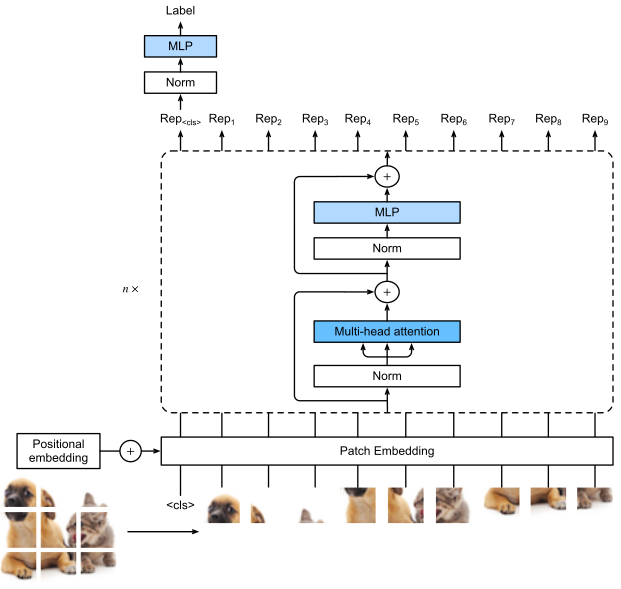
Consider an input image with height \(h\), width \(w\), and \(c\) channels. With patch height and width both set to \(p\), the image is split into a sequence of \(m = hw/p^2\) patches, each flattened to a vector of length \(cp^2\). A special “<cls>” (class) token and the \(m\) flattened patches are linearly projected into \(m + 1\) vectors and summed with learnable positional embeddings. From here on the model is the encoder wiring of Section 11.4: a stack of transformer blocks with no causal mask, every token attending to every other, mapping \(m + 1\) input vectors to \(m + 1\) output representations of the same dimension. Since the “<cls>” token attends to all the image patches, its representation at the output of the stack summarizes the whole image and is the one the classification head reads.
Splitting an image into patches and linearly projecting the flattened patches sounds like two operations, but they combine into one: a convolution whose kernel size and stride both equal the patch size. Each output position of such a convolution sees exactly one patch and computes exactly its linear projection.
class PatchEmbedding(nn.Module):
    """Image-to-sequence stem of the vision transformer."""
    def __init__(self, img_size=96, patch_size=16, num_hiddens=512):
        super().__init__()
        def _make_tuple(x):
            if not isinstance(x, (list, tuple)):
                return (x, x)
            return x
        img_size, patch_size = _make_tuple(img_size), _make_tuple(patch_size)
        # A partial trailing patch would silently shrink the token grid
        assert img_size[0] % patch_size[0] == 0 and \
            img_size[1] % patch_size[1] == 0, \
            'image size must be divisible by the patch size'
        self.num_patches = (img_size[0] // patch_size[0]) * (
            img_size[1] // patch_size[1])
        self.conv = nn.LazyConv2d(num_hiddens, kernel_size=patch_size,
                                  stride=patch_size)

    def forward(self, X):
        # Output shape: (batch size, no. of patches, no. of channels)
        return self.conv(X).flatten(2).transpose(1, 2)
class PatchEmbedding(nnx.Module):
"""Image-to-sequence stem of the vision transformer."""
def __init__(self, img_size=96, patch_size=16, num_hiddens=512,
num_channels=3, rngs=None):
rngs = nnx.Rngs(0) if rngs is None else rngs
def _make_tuple(x):
if not isinstance(x, (list, tuple)):
return (x, x)
return x
img_size, patch_size = _make_tuple(img_size), _make_tuple(patch_size)
# A partial trailing patch would silently shrink the token grid
assert img_size[0] % patch_size[0] == 0 and \
img_size[1] % patch_size[1] == 0, \
'image size must be divisible by the patch size'
self.num_patches = (img_size[0] // patch_size[0]) * (
img_size[1] // patch_size[1])
self.conv = nnx.Conv(num_channels, num_hiddens, kernel_size=patch_size,
strides=patch_size, padding='VALID', rngs=rngs)
def __call__(self, X):
# Output shape: (batch size, no. of patches, no. of channels)
X = self.conv(X)
return X.reshape((X.shape[0], -1, X.shape[3]))In the following example, taking images with height and width of img_size as inputs, the patch embedding outputs (img_size//patch_size)**2 patches that are linearly projected to vectors of length num_hiddens.
img_size, patch_size, num_hiddens, batch_size = 96, 16, 512, 4
patch_emb = PatchEmbedding(img_size, patch_size, num_hiddens)
X = d2l.zeros(batch_size, 3, img_size, img_size)
d2l.check_shape(patch_emb(X),
                (batch_size, (img_size//patch_size)**2, num_hiddens))
img_size, patch_size, num_hiddens, batch_size = 96, 16, 512, 4
patch_emb = PatchEmbedding(img_size, patch_size, num_hiddens)
X = d2l.zeros((batch_size, img_size, img_size, 3))
d2l.check_shape(patch_emb(X),
(batch_size, (img_size//patch_size)**2, num_hiddens))This patch projection is the interface between the image and the transformer. Subsequent blocks process the patch vectors in the same form as token embeddings.
11.5.2 The Vision Transformer Block
The body of the model is the transformer block of Section 11.1 in its pre-norm configuration: normalization sits on each branch, right before multi-head attention and before the MLP, and the residual stream runs uninterrupted. ViT adopted this arrangement as analyses began to establish its training advantages (Baevski and Auli 2018; Wang et al. 2019; Xiong et al. 2020). Pre-norm subsequently became common in transformer architectures.
Two details are specific to the vision variant. The MLP uses the Gaussian error linear unit (GELU), a smooth relative of ReLU (Hendrycks and Gimpel 2016), and applies dropout after each of its two linear layers. Dropout is retained in the ViT training recipe, unlike in many large language-model recipes. And because every patch is a valid token that may look at every other, the block needs no mask: the valid_lens argument of the d2l.MultiHeadAttention from Section 10.3 stays None throughout this section.
class ViTBlock(nn.Module):
    """Pre-norm transformer block with a GELU MLP."""
    def __init__(self, num_hiddens, mlp_num_hiddens, num_heads, dropout,
                 use_bias=False):
        super().__init__()
        self.ln1 = nn.LayerNorm(num_hiddens)
        self.attention = d2l.MultiHeadAttention(num_hiddens, num_heads,
                                                dropout, use_bias)
        self.ln2 = nn.LayerNorm(num_hiddens)
        self.mlp = nn.Sequential(
            nn.LazyLinear(mlp_num_hiddens), nn.GELU(), nn.Dropout(dropout),
            nn.LazyLinear(num_hiddens), nn.Dropout(dropout))

    def forward(self, X, valid_lens=None):
        X = X + self.attention(*([self.ln1(X)] * 3), valid_lens)
        return X + self.mlp(self.ln2(X))
class ViTBlock(nnx.Module):
"""Pre-norm transformer block with a GELU MLP."""
def __init__(self, num_hiddens, mlp_num_hiddens, num_heads, dropout,
use_bias=False, rngs=None):
rngs = nnx.Rngs(params=0, dropout=1) if rngs is None else rngs
self.ln1 = nnx.LayerNorm(num_hiddens, rngs=rngs)
self.attention = d2l.MultiHeadAttention(
num_hiddens, num_heads, dropout, use_bias, rngs=rngs)
self.ln2 = nnx.LayerNorm(num_hiddens, rngs=rngs)
self.mlp = nnx.Sequential(
nnx.Linear(num_hiddens, mlp_num_hiddens, rngs=rngs), nnx.gelu,
nnx.Dropout(dropout, rngs=rngs),
nnx.Linear(mlp_num_hiddens, num_hiddens, rngs=rngs),
nnx.Dropout(dropout, rngs=rngs))
def __call__(self, X, valid_lens=None):
X_norm = self.ln1(X)
X = X + self.attention(X_norm, X_norm, X_norm, valid_lens)[0]
return X + self.mlp(self.ln2(X))As with every transformer block, the output shape equals the input shape, so the blocks can be stacked directly.
X = d2l.ones((2, 100, 24))
encoder_blk = ViTBlock(24, 48, 8, 0.5)
encoder_blk.eval()
d2l.check_shape(encoder_blk(X), X.shape)
X = d2l.ones((2, 100, 24))
encoder_blk = ViTBlock(24, 48, 8, 0.5)
d2l.check_shape(nnx.view(encoder_blk, deterministic=True)(X), X.shape)11.5.3 The Full Model
Assembling the pieces takes one class. Input images pass through a PatchEmbedding instance; a learnable “<cls>” token embedding, initialized to zeros, is prepended to the resulting sequence. The sum with the positional embeddings goes through dropout, then through num_blks stacked ViTBlock instances, and finally the head projects the “<cls>” token’s representation to the class logits.
The positional embeddings must represent a two-dimensional grid. The sinusoidal and rotary constructions of Section 10.4 encode positions along a line, but a patch has a row and a column, and it is not obvious what a hand-designed two-dimensional code should look like. ViT sidesteps the question: the position embeddings are a freely learnable parameter, initialized to small Gaussian noise as in the original recipe, one vector per sequence position. At initialization, the model therefore does not encode that patch 7 lies directly left of patch 8 and directly above patch 13; the patches enter as an unordered set of vectors. Whatever spatial structure the trained model uses, it must discover during training. We will check how far it gets.
class ViT(d2l.Classifier):
    """Vision transformer."""
    def __init__(self, img_size, patch_size, num_hiddens, mlp_num_hiddens,
                 num_heads, num_blks, emb_dropout, blk_dropout, lr=0.1,
                 use_bias=False, num_classes=10):
        super().__init__()
        self.save_hyperparameters()
        self.patch_embedding = PatchEmbedding(
            img_size, patch_size, num_hiddens)
        self.cls_token = nn.Parameter(d2l.zeros(1, 1, num_hiddens))
        num_steps = self.patch_embedding.num_patches + 1  # Add the cls token
        # Positional embeddings are learnable, initialized to small noise
        self.pos_embedding = nn.Parameter(
            torch.randn(1, num_steps, num_hiddens) * 0.02)
        self.dropout = nn.Dropout(emb_dropout)
        self.blks = nn.Sequential()
        for i in range(num_blks):
            self.blks.add_module(f"{i}", ViTBlock(
                num_hiddens, mlp_num_hiddens, num_heads, blk_dropout,
                use_bias))
        self.head = nn.Sequential(nn.LayerNorm(num_hiddens),
                                  nn.Linear(num_hiddens, num_classes))

    def forward(self, X):
        X = self.patch_embedding(X)
        X = d2l.concat((self.cls_token.expand(X.shape[0], -1, -1), X), 1)
        X = self.dropout(X + self.pos_embedding)
        for blk in self.blks:
            X = blk(X)
        return self.head(X[:, 0])
class ViT(d2l.Classifier):
"""Vision transformer."""
def __init__(self, img_size, patch_size, num_hiddens, mlp_num_hiddens,
num_heads, num_blks, emb_dropout, blk_dropout, lr=0.1,
use_bias=False, num_classes=10, num_channels=1, rngs=None):
super().__init__()
self.save_hyperparameters(ignore=['rngs'])
rngs = nnx.Rngs(params=0, dropout=1) if rngs is None else rngs
self.patch_embedding = PatchEmbedding(
img_size, patch_size, num_hiddens, num_channels, rngs=rngs)
self.cls_token = nnx.Param(jnp.zeros((1, 1, num_hiddens)))
num_steps = self.patch_embedding.num_patches + 1 # Add the cls token
# Positional embeddings are learnable, initialized to small noise
self.pos_embedding = nnx.Param(
rngs.params.normal((1, num_steps, num_hiddens)) * 0.02)
self.embedding_dropout = nnx.Dropout(emb_dropout, rngs=rngs)
self.blks = nnx.List([
ViTBlock(num_hiddens, mlp_num_hiddens, num_heads, blk_dropout,
use_bias, rngs=rngs) for _ in range(num_blks)])
self.head = nnx.Sequential(
nnx.LayerNorm(num_hiddens, rngs=rngs),
nnx.Linear(num_hiddens, num_classes, rngs=rngs))
def forward(self, X):
X = self.patch_embedding(X)
X = d2l.concat((jnp.tile(self.cls_token, (X.shape[0], 1, 1)), X), 1)
X = self.embedding_dropout(X + self.pos_embedding)
for blk in self.blks:
X = blk(X)
return self.head(X[:, 0])Why read the class from the “<cls>” token rather than, say, averaging all the patch representations? Both work. The extra token is a learned querying device (through two rounds of attention it can ask for whatever evidence the classification needs), and it matches the original recipe; the exercises invite you to try the averaging variant.
11.5.4 Training and What the Model Learns
11.5.4.1 A First Run
We train a small ViT on Fashion-MNIST, resized to \(96 \times 96\) so that a \(16 \times 16\) patch size yields \(6 \times 6 = 36\) patch tokens. The recipe is deliberately the one used for CNNs in Chapter 7: 10 epochs, batch size 128, plain SGD.
img_size, patch_size = 96, 16
num_hiddens, mlp_num_hiddens, num_heads, num_blks = 512, 2048, 8, 2
emb_dropout, blk_dropout, lr = 0.1, 0.1, 0.1
model = ViT(img_size, patch_size, num_hiddens, mlp_num_hiddens, num_heads,
            num_blks, emb_dropout, blk_dropout, lr)
trainer = d2l.Trainer(max_epochs=10, num_gpus=1)
data = d2l.FashionMNIST(batch_size=128, resize=(img_size, img_size))
trainer.fit(model, data)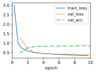
img_size, patch_size = 96, 16
num_hiddens, mlp_num_hiddens, num_heads, num_blks = 512, 2048, 8, 2
emb_dropout, blk_dropout, lr = 0.1, 0.1, 0.1
model = ViT(img_size, patch_size, num_hiddens, mlp_num_hiddens, num_heads,
            num_blks, emb_dropout, blk_dropout, lr)
trainer = d2l.Trainer(max_epochs=10, num_gpus=1)
data = d2l.FashionMNIST(batch_size=128, resize=(img_size, img_size))
trainer.fit(model, data)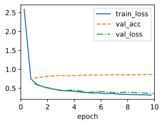
if tab.selected('pytorch'):
    vit_params = sum(p.numel() for p in model.parameters()
                     if p.requires_grad)
if tab.selected('jax'):
    vit_params = sum(p.size for p in
                     jax.tree.leaves(nnx.state(model, nnx.Param)))
vit_acc = float(model.board.data['val_acc'][-1].y)
print(f'ViT: {vit_params/1e6:.1f}M parameters, '
      f'validation accuracy {vit_acc:.2f}')
ViT: 6.5M parameters, validation accuracy 0.85if tab.selected('pytorch'):
vit_params = sum(p.numel() for p in model.parameters()
if p.requires_grad)
if tab.selected('jax'):
vit_params = sum(p.size for p in
jax.tree.leaves(nnx.state(model, nnx.Param)))
vit_acc = float(model.board.data['val_acc'][-1].y)
print(f'ViT: {vit_params/1e6:.1f}M parameters, '
f'validation accuracy {vit_acc:.2f}')ViT: 6.5M parameters, validation accuracy 0.87The model trains without drama to a validation accuracy of about 86–87%. Keep that number in mind; we will shortly see what a CNN of the same size does with the same ten epochs.
11.5.4.2 Do the Position Embeddings Discover the Grid?
First, though, let us look inside. The position embeddings started as noise, and nothing in the training signal ever named a row or a column. In fully trained ViTs the embeddings famously end up reflecting the grid anyway: in the original paper’s analysis, each position’s embedding is most similar to the embeddings of its spatial neighbors, with clear row and column bands — two-dimensional structure induced by the data alone (Dosovitskiy et al. 2021). Does our small model already show this? For each of the 36 patch positions we take its embedding vector, compute its cosine similarity with the embeddings of all 36 positions, and reshape those similarities into the \(6 \times 6\) patch grid. Laying out the 36 resulting maps in the grid itself gives a picture in which position \((i, j)\) of the big grid shows how similar position \((i, j)\)’s embedding is to everywhere else’s.
P = model.pos_embedding[0, 1:].detach().cpu()  # (36, 512): drop the cls slot
P = P / P.norm(dim=1, keepdim=True)
sim = P @ P.T                                  # Pairwise cosine similarities
coords = torch.stack(torch.meshgrid(
    torch.arange(6), torch.arange(6), indexing='ij'), -1).reshape(36, 2)
dist = (coords[:, None] - coords[None]).abs().amax(-1)  # Chebyshev distance
print(f'mean cosine similarity: grid neighbors {sim[dist == 1].mean():.2f}, '
      f'distant positions {sim[dist >= 3].mean():.2f}')
d2l.show_heatmaps(sim.reshape(6, 6, 6, 6), xlabel='', ylabel='',
                  figsize=(5, 5), cmap='Reds')
mean cosine similarity: grid neighbors 0.05, distant positions -0.02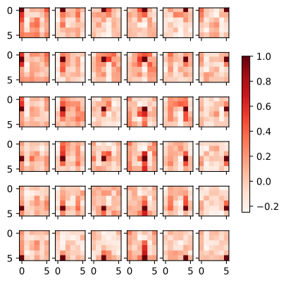
P = model.pos_embedding[0, 1:]                 # (36, 512): drop the cls slot
P = P / jnp.linalg.norm(P, axis=1, keepdims=True)
sim = P @ P.T                                  # Pairwise cosine similarities
coords = jnp.stack(jnp.meshgrid(
    jnp.arange(6), jnp.arange(6), indexing='ij'), -1).reshape(36, 2)
dist = jnp.abs(coords[:, None] - coords[None]).max(-1)  # Chebyshev distance
print(f'mean cosine similarity: grid neighbors {sim[dist == 1].mean():.2f}, '
      f'distant positions {sim[dist >= 3].mean():.2f}')
d2l.show_heatmaps(sim.reshape(6, 6, 6, 6), xlabel='', ylabel='',
                  figsize=(5, 5), cmap='Reds')
mean cosine similarity: grid neighbors 0.05, distant positions -0.03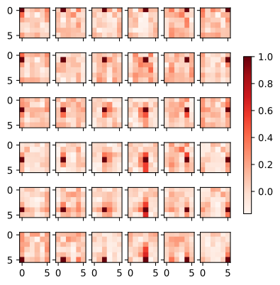
Each map’s darkest cell is its own position, which is mere self-similarity; the surrounding similarities determine whether spatial structure has emerged. After ten epochs, they show only weak traces of the grid. The printed statistic makes it precise: averaged over positions, immediate grid neighbors score slightly positive cosine similarity while distant positions score slightly negative, and several maps show a diffuse halo around their own cell or a weak band along their own column — but the values are small and the pattern is easy to miss without the summary statistics. Compare this with the crisp row-and-column structure that emerges in fully trained ViTs, and the state of our model is clear: the embeddings contain weak evidence of the spatial geometry that was not encoded at initialization. The next comparison uses an architecture that encodes this geometry directly.
11.5.4.3 A Convolutional Baseline at the Same Budget
The ViT above has about 6.5 million parameters. To make the inductive-bias comparison fair we build a CNN with the same budget, from the Residual blocks of Section 7.4: the familiar \(7 \times 7\) stem, then seven residual blocks whose channel widths are chosen so that the total lands at the ViT’s parameter count. It trains on the identical data pipeline for the identical ten epochs, with the learning rate that Section 7.4 established for this family.
class CompactResNet(d2l.Classifier):
    """A ResNet-style CNN parameter-matched to the ViT above."""
    def __init__(self, lr=0.01, num_classes=10):
        super().__init__()
        self.save_hyperparameters()
        self.net = nn.Sequential(
            nn.LazyConv2d(64, kernel_size=7, stride=2, padding=3),
            nn.LazyBatchNorm2d(), nn.ReLU(),
            nn.MaxPool2d(kernel_size=3, stride=2, padding=1),
            d2l.Residual(64), d2l.Residual(64),
            d2l.Residual(128, strides=2), d2l.Residual(128),
            d2l.Residual(256, strides=2), d2l.Residual(256),
            d2l.Residual(512, strides=2),
            nn.AdaptiveAvgPool2d((1, 1)), nn.Flatten(),
            nn.LazyLinear(num_classes))

    def forward(self, X):
        return self.net(X)
class CompactResNet(d2l.Classifier):
"""A ResNet-style CNN parameter-matched to the ViT above."""
def __init__(self, lr=0.01, num_classes=10, rngs=None):
super().__init__()
self.save_hyperparameters(ignore=['rngs'])
rngs = nnx.Rngs(0) if rngs is None else rngs
self.net = nnx.Sequential(
nnx.Conv(1, 64, kernel_size=(7, 7), strides=(2, 2),
padding='same', rngs=rngs),
nnx.BatchNorm(64, rngs=rngs), nnx.relu,
lambda x: nnx.max_pool(x, window_shape=(3, 3),
strides=(2, 2), padding='same'),
d2l.Residual(64, in_channels=64, rngs=rngs),
d2l.Residual(64, in_channels=64, rngs=rngs),
d2l.Residual(128, strides=(2, 2), in_channels=64, rngs=rngs),
d2l.Residual(128, in_channels=128, rngs=rngs),
d2l.Residual(256, strides=(2, 2), in_channels=128, rngs=rngs),
d2l.Residual(256, in_channels=256, rngs=rngs),
d2l.Residual(512, strides=(2, 2), in_channels=256, rngs=rngs),
lambda x: x.mean(axis=(1, 2)),
nnx.Linear(512, num_classes, rngs=rngs))
def forward(self, X):
return self.net(X)cnn = CompactResNet()
trainer = d2l.Trainer(max_epochs=10, num_gpus=1)
trainer.fit(cnn, data)
if tab.selected('pytorch'):
cnn_params = sum(p.numel() for p in cnn.parameters() if p.requires_grad)
if tab.selected('jax'):
cnn_params = sum(p.size for p in
jax.tree.leaves(nnx.state(cnn, nnx.Param)))
cnn_acc = float(cnn.board.data['val_acc'][-1].y)
print(f'CNN: {cnn_params/1e6:.1f}M parameters, '
f'validation accuracy {cnn_acc:.2f}')
print(f'ViT: {vit_params/1e6:.1f}M parameters, '
f'validation accuracy {vit_acc:.2f}')CNN: 6.5M parameters, validation accuracy 0.91
ViT: 6.5M parameters, validation accuracy 0.85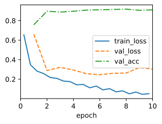
cnn = CompactResNet()
trainer = d2l.Trainer(max_epochs=10, num_gpus=1)
trainer.fit(cnn, data)
if tab.selected('pytorch'):
    cnn_params = sum(p.numel() for p in cnn.parameters() if p.requires_grad)
if tab.selected('jax'):
    cnn_params = sum(p.size for p in
                     jax.tree.leaves(nnx.state(cnn, nnx.Param)))
cnn_acc = float(cnn.board.data['val_acc'][-1].y)
print(f'CNN: {cnn_params/1e6:.1f}M parameters, '
      f'validation accuracy {cnn_acc:.2f}')
print(f'ViT: {vit_params/1e6:.1f}M parameters, '
      f'validation accuracy {vit_acc:.2f}')
CNN: 6.5M parameters, validation accuracy 0.91
ViT: 6.5M parameters, validation accuracy 0.87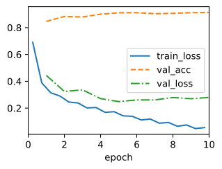
At the same parameter count, with the same data and number of epochs, the CNN performs better by several points, about 90–92% against the ViT’s 86–87%, a margin well beyond the run-to-run noise of these ten-epoch runs. The result is consistent with an advantage from the convolutional prior at this scale, although the comparison does not isolate that cause. Locality and translation equivariance are a strong prior the CNN has by construction; the transformer must infer both from data. After ten epochs, the position-embedding similarities show only weak grid structure. This experiment compares two models on Fashion-MNIST; it does not rank vision architectures generally. The discussion below considers published results under much larger pretraining protocols.
11.5.5 Summary
A vision transformer converts an image into a sequence with a strided convolution and processes the sequence with an encoder stack. Relative to the text model, the new components are the patch embedding, the “<cls>” readout, and learned position embeddings.
At matched parameter count, data, and training budget, the CNN performs better because convolution builds in locality and translation equivariance (Section 6.1), while the transformer must extract both from 60,000 images. Large-scale published comparisons reach a different outcome. Under the JFT-300M pretraining, model-size, and fine-tuning protocol of Dosovitskiy et al. (2021), ViT variants exceed the cited ResNet-based baselines. This result reflects the complete protocol, not data scale alone. DeiT showed that augmentation and distillation can make ViTs competitive on ImageNet-1k without JFT pretraining (Touvron et al. 2021). A complementary line, Swin transformers, reinstates convolution-like priors (local attention windows, hierarchical resolution) partly to escape the quadratic cost of global attention (Section 10.5) at high resolution (Liu et al. 2021).
Plain ViT encoders are used in several vision–language model families, including CLIP (Radford et al. 2021), while hierarchical transformers and convolutional backbones remain common in classification, detection, and segmentation. The appropriate backbone depends on the task, training protocol, and deployment constraints; Chapter 20 develops these applications.
11.5.6 Exercises
- How does the value of
img_sizeaffect training time? Predict what halvingpatch_sizeto 8 does to the sequence length and to the cost of an attention layer (Section 10.5), then measure the time per epoch. - Instead of projecting the “<cls>” token representation to the output, project the averaged patch representations. Implement this change and see how it affects the accuracy.
- Add data augmentation — random horizontal flips and random crops — to the training pipeline and retrain both the ViT and the CNN. Does the gap between them shrink? Relate what you find to the DeiT recipe.
- Apply a fixed random permutation to the 36 patch tokens at test time (after patch embedding, leaving the position embeddings in place) and measure the accuracy of the trained ViT. What does the size of the drop tell you about how much the model relies on its position embeddings?
- To fine-tune a trained ViT at a higher resolution, the standard trick is to interpolate its position embeddings: reshape the \(36\) patch embeddings to \(6 \times 6 \times d\), resize spatially to the new grid, and flatten back. Implement this for \(144 \times 144\) inputs (a \(9 \times 9\) grid) and verify that the model still classifies far better than chance without any retraining.