%matplotlib inline
from d2l import torch as d2l
import numpy as np26.1 Gradient-Based Optimization
An optimization step has two distinct parts: a direction and a distance. A gradient supplies the locally steepest direction, while smoothness, a line search, or a curvature model determines how far that direction can be trusted. This section develops that distinction first, then studies conditioning, momentum, stochastic gradients, Newton’s method, quasi-Newton updates, and trust regions.
We assume familiarity with gradients, directional derivatives, Hessians, and eigenvalues from Section 25.2 and Section 24.2. The convex convergence results stated here are proved in Section 26.3. Implementations use NumPy so that each update can be compared directly with its defining equation.
%matplotlib inline
from d2l import tensorflow as d2l
import numpy as np%matplotlib inline
from d2l import jax as d2l
import numpy as np%matplotlib inline
from d2l import mxnet as d2l
import numpy as np26.1.1 Descent Directions
At a point \(\mathbf{x}\), the first optimization choice is the update direction. The multivariable calculus of Section 25.2 supplies the local model. For a differentiable \(f : \mathbb{R}^n \to \mathbb{R}\), a small step of size \(\eta > 0\) along a direction \(\mathbf{d}\) changes the value by
\[ f(\mathbf{x} + \eta\,\mathbf{d}) = f(\mathbf{x}) + \eta\, \nabla f(\mathbf{x})^\top \mathbf{d} + o(\eta), \]
so the directional derivative \(\nabla f(\mathbf{x})^\top \mathbf{d}\) determines the change predicted by the first-order model. Call \(\mathbf{d}\) a descent direction at \(\mathbf{x}\) if \(\nabla f(\mathbf{x})^\top \mathbf{d} < 0\). A negative slope in the model forces a genuine decrease of \(f\) for all sufficiently small steps, and among all unit directions there is a unique steepest one.
Proposition (descent directions, and the steepest one). Let \(f\) be differentiable at \(\mathbf{x}\) with \(\nabla f(\mathbf{x}) \neq \mathbf{0}\).
- If \(\nabla f(\mathbf{x})^\top \mathbf{d} < 0\), then \(f(\mathbf{x} + \eta\,\mathbf{d}) < f(\mathbf{x})\) for every sufficiently small \(\eta > 0\).
- Among unit vectors, the directional derivative is minimized uniquely by the normalized negative gradient:
\[ \min_{\|\mathbf{d}\| = 1} \nabla f(\mathbf{x})^\top \mathbf{d} = -\|\nabla f(\mathbf{x})\|, \qquad \textrm{attained only at } \mathbf{d} = -\frac{\nabla f(\mathbf{x})}{\|\nabla f(\mathbf{x})\|}. \tag{26.1.1}\]
Proof. For the first claim, the function \(\varphi(\eta) = f(\mathbf{x} + \eta\,\mathbf{d})\) has \(\varphi'(0) = \nabla f(\mathbf{x})^\top \mathbf{d} < 0\) by the chain rule, so the difference quotient \((\varphi(\eta) - \varphi(0))/\eta\) is negative for all small \(\eta > 0\), i.e. \(\varphi(\eta) < \varphi(0)\). The second claim is the steepest-descent proposition proved by Cauchy–Schwarz in Section 25.2. \(\blacksquare\)
Statement 2 explains why gradient descent follows \(-\nabla f\). Locally, descent directions form the open half-space of vectors making an acute angle with \(-\nabla f\). For any such direction, differentiability guarantees a decrease only for sufficiently small positive steps; a finite step requires a smoothness bound or a line-search test. For any positive-definite matrix \(B\), every vector in the family \(\mathbf{d} = -B\,\nabla f(\mathbf{x})\) is a descent direction (Exercise 2). Newton’s method and preconditioned optimizers are instances of this family, with \(B\) encoding curvature; we return to them in Section 26.1.5.3. The following cell evaluates the proposition on this section’s running example, \(f(x, y) = \tfrac12(x^2 + 10\,y^2)\): it compares the first-order slope and the actual decrease along several unit directions, then scans \(3600\) directions to confirm that the most negative slope occurs at \(-\nabla f / \|\nabla f\|\).
def f(v):
    return 0.5 * (v[0]**2 + 10 * v[1]**2)

def grad(v):
    return np.array([v[0], 10 * v[1]])

x = np.array([2.0, 1.0])
g = grad(x)
steepest = -g / np.linalg.norm(g)
candidates = [('steepest -grad/|grad|', steepest),
              ('diagonal -(1,1)/sqrt(2)', -np.ones(2) / np.sqrt(2)),
              ('axis     (-1,0)', np.array([-1.0, 0.0])),
              ('uphill   +(1,1)/sqrt(2)', np.ones(2) / np.sqrt(2))]
eta = 0.01
for name, d in candidates:
    print(f'{name}:  slope = {g @ d:+8.4f},  '
          f'f(x + eta d) - f(x) = {f(x + eta * d) - f(x):+.6f}')
thetas = np.linspace(0.0, 2 * np.pi, 3601)
dirs = np.stack([np.cos(thetas), np.sin(thetas)])
best = dirs[:, np.argmin(g @ dirs)]
print('best of 3600 sampled unit directions:', best.round(4),
      ' vs  -grad/|grad| =', steepest.round(4))
steepest -grad/|grad|: slope = -10.1980, f(x + eta d) - f(x) = -0.101498
diagonal -(1,1)/sqrt(2): slope = -8.4853, f(x + eta d) - f(x) = -0.084578
axis (-1,0): slope = -2.0000, f(x + eta d) - f(x) = -0.019950
uphill +(1,1)/sqrt(2): slope = +8.4853, f(x + eta d) - f(x) = +0.085128
best of 3600 sampled unit directions: [-0.1959 -0.9806] vs -grad/|grad| = [-0.1961 -0.9806]Every direction with negative slope lowers \(f\) for the tested step. The axis direction has slope \(-2.0\), five times smaller in magnitude than the steepest slope \(-10.198\). The unit-circle scan returns \((-0.196, -0.981)\), the normalized negative gradient, to grid resolution. “Steepest” describes the local first-order change, not multistep convergence speed. On an ill-conditioned quadratic, steepest descent can oscillate across high-curvature directions; momentum (Section 26.1.4) reduces this effect.
26.1.2 Gradient Descent and Smoothness
26.1.2.1 The Iteration and the Smoothness Assumption
Gradient descent iterates the steepest step with a fixed step size (learning rate) \(\eta > 0\):
\[ \mathbf{x}_{k+1} = \mathbf{x}_k - \eta\, \nabla f(\mathbf{x}_k). \tag{26.1.2}\]
The first-order model justified the direction; it says nothing about how far to trust that direction. The first-order approximation at \(\mathbf{x}_k\) becomes less accurate away from that point. The additional assumption bounds how quickly the gradient can change. We say \(f\) is \(L\)-smooth if its gradient is \(L\)-Lipschitz,
\[ \|\nabla f(\mathbf{x}) - \nabla f(\mathbf{y})\| \;\le\; L\, \|\mathbf{x} - \mathbf{y}\| \qquad \textrm{for all } \mathbf{x}, \mathbf{y}, \tag{26.1.3}\]
which for twice-differentiable \(f\) is equivalent to every Hessian eigenvalue lying in \([-L, L]\): bounded eigenvalues give Equation 26.1.3 by integrating the Hessian along the segment from \(\mathbf{x}\) to \(\mathbf{y}\) (the same device as in the proof below), and the converse is a mean-value argument we leave to the reader. Either way, the curvature is bounded by \(L\) in every direction. Smoothness converts the first-order model into a one-sided guarantee: a quadratic upper bound
\[ f(\mathbf{y}) \;\le\; f(\mathbf{x}) + \nabla f(\mathbf{x})^\top (\mathbf{y} - \mathbf{x}) + \tfrac{L}{2}\, \|\mathbf{y} - \mathbf{x}\|^2 \tag{26.1.4}\]
that is tight at \(\mathbf{x}\). The one-dimensional version of this bound (and the figure that illustrates the next proof) is Figure 25.1.3 in Section 25.1: the value of \(f\) at the upper bound’s minimizer cannot exceed the bound there, so minimizing the bound provides a guaranteed decrease in \(f\).
26.1.2.2 The Descent Lemma
Proposition (descent lemma). If \(f\) is \(L\)-smooth, then the gradient step Equation 26.1.2 satisfies
\[ f(\mathbf{x}_{k+1}) \;\le\; f(\mathbf{x}_k) - \eta \left(1 - \tfrac{L\eta}{2}\right) \|\nabla f(\mathbf{x}_k)\|^2. \tag{26.1.5}\]
In particular \(f\) strictly decreases whenever \(0 < \eta < 2/L\) and \(\nabla f(\mathbf{x}_k) \neq \mathbf{0}\), and the guaranteed decrease is largest at \(\eta = 1/L\), where it reads \(f(\mathbf{x}_{k+1}) \le f(\mathbf{x}_k) - \tfrac{1}{2L}\|\nabla f(\mathbf{x}_k)\|^2\).
Proof. First the ceiling Equation 26.1.4. Restrict \(f\) to the segment, \(g(t) = f(\mathbf{x} + t(\mathbf{y} - \mathbf{x}))\) for \(t \in [0, 1]\), so that \(g'(t) = \nabla f(\mathbf{x} + t(\mathbf{y}-\mathbf{x}))^\top (\mathbf{y} - \mathbf{x})\). By the fundamental theorem of calculus and then Cauchy–Schwarz with the Lipschitz bound Equation 26.1.3,
\[ \begin{aligned} f(\mathbf{y}) - f(\mathbf{x}) - \nabla f(\mathbf{x})^\top (\mathbf{y}-\mathbf{x}) &= \int_0^1 \big(\nabla f(\mathbf{x} + t(\mathbf{y}-\mathbf{x})) - \nabla f(\mathbf{x})\big)^\top (\mathbf{y}-\mathbf{x})\, dt \\ &\le \int_0^1 L\,t\, \|\mathbf{y}-\mathbf{x}\|^2\, dt = \tfrac{L}{2}\|\mathbf{y}-\mathbf{x}\|^2, \end{aligned} \]
which is the same argument as the 1-D proof in Section 25.1, applied along the segment. Now insert the gradient step \(\mathbf{y} = \mathbf{x}_k - \eta \nabla f(\mathbf{x}_k)\):
\[ f(\mathbf{x}_{k+1}) \;\le\; f(\mathbf{x}_k) - \eta\,\|\nabla f(\mathbf{x}_k)\|^2 + \tfrac{L}{2}\,\eta^2\, \|\nabla f(\mathbf{x}_k)\|^2, \]
and the bracket \(\eta(1 - L\eta/2)\) is positive exactly for \(\eta < 2/L\) and maximized at \(\eta = 1/L\). \(\blacksquare\)
The assumption is global \(L\)-smoothness on the region containing the step. The conclusion is a finite decrease for \(0<\eta<2/L\), not global convergence by itself. In practice, a conservative smoothness estimate or backtracking line search supplies the missing step-length control.
The first-order decrease is \(\eta\,\|\nabla f\|^2\), while the curvature error is at most \(\tfrac{L}{2}\eta^2\,\|\nabla f\|^2\). The former grows linearly in \(\eta\) and the latter quadratically, so sufficiently short steps decrease the objective; the limiting value is \(\eta = 2/L\). This comparison underlies the learning-rate arguments used throughout the book.
26.1.2.3 Guarantees Without Convexity
The lemma alone, with no convexity, yields the standard smooth nonconvex benchmark for neural-network optimization. It is an idealized model rather than a theorem about every network: ReLU objectives are nonsmooth, and a useful \(L\)-smooth bound may hold only locally or along a particular trajectory.
Proposition (gradient descent finds approximate stationary points). Let \(f\) be \(L\)-smooth and bounded below by \(f^\star\), and run Equation 26.1.2 with \(\eta = 1/L\). Then for every \(K \ge 1\),
\[ \min_{0 \le k < K} \|\nabla f(\mathbf{x}_k)\|^2 \;\le\; \frac{2L\,\big(f(\mathbf{x}_0) - f^\star\big)}{K}. \tag{26.1.6}\]
Proof. At \(\eta = 1/L\) the descent lemma reads \(\|\nabla f(\mathbf{x}_k)\|^2 \le 2L\,(f(\mathbf{x}_k) - f(\mathbf{x}_{k+1}))\). Sum over \(k = 0, \ldots, K-1\); the right side telescopes to \(2L\,(f(\mathbf{x}_0) - f(\mathbf{x}_K)) \le 2L\,(f(\mathbf{x}_0) - f^\star)\). The smallest of \(K\) numbers is at most their average. \(\blacksquare\)
Within this smooth model the hypotheses are modest: a loss bounded below and a finite smoothness constant on the region traversed by the iterates. No convexity or unique minimum is required, and some iterate among the first \(K\) has squared gradient norm \(O(1/K)\). The result is a useful reference point for neural-network training, but it guarantees a small gradient only when those smoothness and step-size assumptions actually hold. What it does not promise is that such a point is a minimum, let alone a global one: it could be a saddle point (Section 25.2) or belong to a flat stationary region. Convexity provides the additional assumptions needed to upgrade “stationary” to “globally optimal”, and the two theorems that do so are stated at the end of Section 26.1.3 and proved in Section 26.3.
26.1.2.4 Backtracking Line Search
The step \(\eta = 1/L\) in the propositions above presumes we know \(L\). We rarely do; worse, the local curvature that matters varies across the loss surface, so a single global constant is both unknown and too conservative. A line search fixes this at runtime: try a step, and demand it achieve a fixed fraction \(c \in (0, 1)\) of the first-order promise, the Armijo condition (also called sufficient decrease) (Armijo 1966)
\[ f\big(\mathbf{x} - \eta\, \nabla f(\mathbf{x})\big) \;\le\; f(\mathbf{x}) - c\,\eta\, \|\nabla f(\mathbf{x})\|^2. \tag{26.1.7}\]
Backtracking starts from an optimistic \(\eta_0\) and halves \(\eta\) until Equation 26.1.7 holds. By the descent lemma the condition is automatic once \(\eta \le 2(1-c)/L\), so the loop terminates after finitely many halvings and always accepts a step \(\eta \ge \min\big(\eta_0,\, (1-c)/L\big)\): within a constant factor of the ideal \(1/L\), found without ever knowing \(L\). The cell compares a fixed step with backtracking on the quartic \(f(x) = \tfrac14 x^4\), whose curvature \(f''(x) = 3x^2\) is large far from the origin and vanishing near it, so no single fixed step is suitable across the full trajectory.
quartic = lambda v: 0.25 * (v ** 4).sum()
quartic_grad = lambda v: v ** 3

x = np.array([3.0])
for _ in range(6):                            # fixed step, too large at x0
    x = x - 0.3 * quartic_grad(x)
print(f'fixed eta = 0.3 from x0 = 3:  |x_6| = {abs(x[0]):.2e}  (diverged)')

x, etas = np.array([3.0]), []
for _ in range(25):                           # backtracking line search
    g = quartic_grad(x)
    eta = 1.0
    while quartic(x - eta * g) > quartic(x) - 0.5 * eta * (g * g).sum():
        eta *= 0.5                            # Armijo fails: halve the step
    x = x - eta * g
    etas.append(eta)
print('accepted steps:', np.array(etas[:8]), '...')
print(f'backtracking from x0 = 3:  f(x_25) = {quartic(x):.2e}  (monotone descent)')
fixed eta = 0.3 from x0 = 3: |x_6| = 6.52e+103 (diverged)
accepted steps: [0.03125 0.0625 0.125 0.25 0.5 1. 1. 1. ] ...
backtracking from x0 = 3: f(x_25) = 1.09e-04 (monotone descent)The fixed step \(\eta = 0.3\) is stable near the minimum but diverges from this initial point: at \(x_0 = 3\) the local curvature is \(f'' = 27\), the local stability ceiling is \(2/27 \approx 0.074\), and six steps later the iterate sits at \(|x_6| \approx 6.5 \times 10^{103}\). Backtracking starts from \(\eta_0 = 1\) and accepts \(0.031\) on the first step, just below the local threshold. As local curvature decreases, the accepted steps increase: \(0.0625, 0.125, 0.25, 0.5, 1.0\). The accepted step is tracking \(2(1-c)/f''(x)\) automatically; a line search is curvature estimation by trial. Deep-learning training rarely uses this procedure because each probe adds an evaluation of \(f\), typically a full forward pass over a batch. Learning-rate schedules are a lower-cost alternative (warmup, decay; Section 9.1 and onward).
26.1.3 The Quadratic Model and the Condition Number
26.1.3.1 Quadratic Objectives as a Local Model
Near a minimum \(\mathbf{x}^\star\), the second-order Taylor expansion of Section 25.2 approximates a smooth function by a quadratic plus a higher-order remainder: \(f(\mathbf{x}) \approx f(\mathbf{x}^\star) + \tfrac12 (\mathbf{x}-\mathbf{x}^\star)^\top H\, (\mathbf{x}-\mathbf{x}^\star)\) with \(H\) the Hessian at the minimum. So we study the model problem
\[ \begin{aligned} f(\mathbf{x}) &= \tfrac12\, \mathbf{x}^\top A\, \mathbf{x}, \qquad A \textrm{ symmetric positive definite,} \\ &\textrm{eigenvalues } 0 < \lambda_{\min} = \lambda_1 \le \cdots \le \lambda_n = \lambda_{\max}, \end{aligned} \]
for which gradient descent can be solved exactly, and the answer turns out to be governed by a single scalar: the condition number \(\kappa = \lambda_{\max} / \lambda_{\min}\) from the introduction (Section 24.3.3.2). Note that \(L = \lambda_{\max}\) here: the smoothness constant of a quadratic is its top eigenvalue.
26.1.3.2 Per-Mode Contraction and the 2/L Ceiling
The gradient is \(\nabla f(\mathbf{x}) = A\mathbf{x}\), so the iteration Equation 26.1.2 is the fixed linear map
\[ \mathbf{x}_{k+1} = (I - \eta A)\, \mathbf{x}_k. \]
Diagonalize: write \(\mathbf{x}_k\) in the orthonormal eigenbasis of \(A\) (Section 24.2) with coefficients \(c_i^{(k)}\). Because \(I - \eta A\) has the same eigenvectors, the coordinates evolve independently:
\[ c_i^{(k+1)} = (1 - \eta \lambda_i)\, c_i^{(k)}, \qquad \textrm{hence} \qquad c_i^{(k)} = (1 - \eta \lambda_i)^k\, c_i^{(0)}. \tag{26.1.8}\]
Gradient descent on a quadratic is \(n\) uncoupled one-dimensional geometric recursions, one per curvature eigenvalue, or “mode.” The factors \(1 - \eta\lambda_i\) determine convergence and speed:
- Convergence requires \(|1 - \eta \lambda_i| < 1\) for every mode, i.e. \(0 < \eta < 2/\lambda_{\max} = 2/L\). This is the stability ceiling: on quadratics, the \(2/L\) that the descent lemma offered as sufficient turns out to be necessary. Above it, the stiffest mode’s factor is below \(-1\), so that coordinate oscillates with increasing amplitude even if other modes converge: divergence along one axis (Exercise 4 has you build this half-converging, half-exploding run).
- Speed is set by the slowest mode: the error norm shrinks like \(\rho(\eta)^k\), where \(\rho(\eta) = \max_i |1 - \eta\lambda_i|\) is the spectral radius of the iteration matrix \(I - \eta A\), its largest eigenvalue magnitude (Section 24.2); the sweep below prints it as its own column.
The cell sweeps \(\eta\) across the ceiling on \(A = \mathrm{diag}(1, 10)\), where \(L = 10\) and the ceiling sits at \(\eta = 0.2\).
A = np.diag([1.0, 10.0])                      # eigenvalues 1 and 10, so L = 10
x0 = np.array([1.0, 1.0])

def run_gd(eta, steps=60):
    xs = [x0]
    for _ in range(steps):
        xs.append(xs[-1] - eta * (A @ xs[-1]))
    return np.array(xs)

print(' eta    |1-eta*1|  |1-eta*10|  spectral radius   |x_60|')
for eta in [0.02, 0.10, 2 / 11, 0.19, 0.20, 0.21]:
    f1, f10 = abs(1 - eta * 1.0), abs(1 - eta * 10.0)
    print(f'{eta:5.3f}    {f1:6.3f}     {f10:6.3f}        {max(f1, f10):6.3f}     '
          f'{np.linalg.norm(run_gd(eta)[-1]):9.1e}')
eta |1-eta*1| |1-eta*10| spectral radius |x_60|
0.020 0.980 0.800 0.980 3.0e-01
0.100 0.900 0.000 0.900 1.8e-03
0.182 0.818 0.818 0.818 8.3e-06
0.190 0.810 0.900 0.900 1.8e-03
0.200 0.800 1.000 1.000 1.0e+00
0.210 0.790 1.100 1.100 3.0e+02Each row of the table represents one step-size regime. The choice \(\eta = 0.02\) is stable but slow (\(\rho = 0.98\); after \(60\) steps the error is still \(0.3\)). At \(\eta = 0.1\) the stiff mode is eliminated in one step (its factor is exactly \(0.000\)) yet the slow mode determines the rate, \(\rho = 0.9\). Note the symmetry: \(\eta = 0.19\) also has \(\rho = 0.9\), but for the opposite reason: its stiff mode oscillates with factor \(-0.9\). Between them, \(\eta = 2/11 \approx 0.182\) balances the two extreme modes and gives the smallest factor (\(\rho = 0.818\), error \(8.3 \times 10^{-6}\)). At the ceiling \(\eta = 0.2\) the stiff mode’s factor is exactly \(-1\): the iterate alternates between \(\pm 1\) on that axis, \(\|\mathbf{x}_{60}\| = 1.0\). At \(\eta = 0.21\), sixty steps increase the error to \(3 \times 10^{2}\).
26.1.3.3 The Optimal Step and the \((\kappa-1)/(\kappa+1)\) Law
Within the stable range, which fixed \(\eta\) is fastest? The sweep already hinted at the answer: balance the two extreme modes.
Proposition (optimal fixed step on a quadratic). For \(f(\mathbf{x}) = \tfrac12 \mathbf{x}^\top A \mathbf{x}\) the convergence factor \(\rho(\eta) = \max_i |1 - \eta\lambda_i|\) is minimized by
\[ \eta^\star = \frac{2}{\lambda_{\min} + \lambda_{\max}}, \qquad \rho(\eta^\star) = \frac{\kappa - 1}{\kappa + 1}, \qquad \kappa = \frac{\lambda_{\max}}{\lambda_{\min}}. \tag{26.1.9}\]
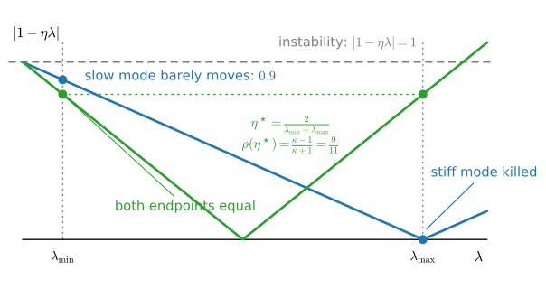
Proof. For fixed \(\eta > 0\), the function \(\lambda \mapsto |1 - \eta\lambda|\) is a V with vertex at \(\lambda = 1/\eta\): it decreases up to the vertex and increases beyond it, so on the interval \([\lambda_{\min}, \lambda_{\max}]\) its maximum sits at an endpoint: \(\rho(\eta) = \max\big(|1 - \eta\lambda_{\min}|,\, |1 - \eta\lambda_{\max}|\big)\). As \(\eta\) grows, the first term \(1 - \eta\lambda_{\min}\) decreases while the second, \(\eta\lambda_{\max} - 1\) (once positive), increases, so the max of the two is minimized where they are equal: \(1 - \eta\lambda_{\min} = \eta\lambda_{\max} - 1\), giving \(\eta^\star = 2/(\lambda_{\min} + \lambda_{\max})\) and \(\rho(\eta^\star) = (\lambda_{\max} - \lambda_{\min})/(\lambda_{\max} + \lambda_{\min}) = (\kappa-1)/(\kappa+1)\). \(\blacksquare\)
Figure 26.1.1 is this proof drawn on the running example: each step size is a “tent” \(|1 - \eta\lambda|\) with vertex at \(\lambda = 1/\eta\), the rate is the taller of the tent’s two values over the extreme eigenvalues, and the best tent is the one whose endpoints are level.
When \(\kappa = 1\) (a perfectly round bowl) the rate is \(0\): one step solves the problem. As \(\kappa\) grows, \((\kappa-1)/(\kappa+1) \approx 1 - 2/\kappa\), so reducing the error by a factor \(\varepsilon\) costs about \(\tfrac{\kappa}{2}\ln\tfrac1\varepsilon\) iterations: the cost of gradient descent is linear in the condition number. The mechanism is a step-size constraint: stability limits the step according to the stiff mode (\(\eta \lesssim 2/L\)), but progress on the slow mode per step is only about \(\eta\,\lambda_{\min} \approx 2/\kappa\). On a quadratic the law is an exact identity, and the cell checks it to the printed precision.
eta_star = 2 / (1.0 + 10.0)                   # 2 / (lambda_min + lambda_max)
xs = run_gd(eta_star, steps=40)
print('per-mode factors x_1/x_0 =', (xs[1] / xs[0]).round(6),
      ' predicted 1 - eta* lambda =', (1 - eta_star * np.diag(A)).round(6))
ratios = np.linalg.norm(xs[1:], axis=1) / np.linalg.norm(xs[:-1], axis=1)
kappa = 10.0
print(f'measured contraction |x_k+1| / |x_k|: min {ratios.min():.6f}, '
      f'max {ratios.max():.6f}')
print(f'predicted (kappa-1)/(kappa+1) = {(kappa - 1) / (kappa + 1):.6f}')
per-mode factors x_1/x_0 = [ 0.818182 -0.818182] predicted 1 - eta* lambda = [ 0.818182 -0.818182]
measured contraction |x_k+1| / |x_k|: min 0.818182, max 0.818182
predicted (kappa-1)/(kappa+1) = 0.818182The two per-mode factors come out as \(+0.818182\) and \(-0.818182\), equal magnitudes and opposite signs, exactly the balance the proof engineered: the slow mode contracts monotonically while the stiff mode alternates in sign, both shrinking by \(9/11\) per step. Consequently the measured contraction of \(\|\mathbf{x}_k\|\) is constant through all forty iterations, \(0.818182\) to six digits, matching \((\kappa-1)/(\kappa+1) = 9/11\). The closed form and the computation agree to the last printed digit.
26.1.3.4 The Valley Picture
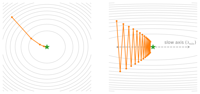
Section 24.3 drew this picture qualitatively (Figure 24.3.5); the optimal-step law is the arithmetic behind it. Figure 26.1.2 replays the geometry on this section’s model problem: on a round bowl (\(\kappa \approx 1\)) one step lands essentially at the minimum, while in a narrow valley (\(\kappa \gg 1\)) the stability-throttled step makes the steep mode overshoot and alternate sign while the flat mode contracts by only \(1 - \eta\lambda_{\min} \approx 1 - 2/\kappa\) per step, and the path zig-zags.
26.1.3.5 The Edge of Stability
A modern measurement changes how this threshold is interpreted. The classical advice is: measure the loss sharpness \(\lambda_{\max}\), then choose \(\eta < 2/\lambda_{\max}\). In some neural-network experiments, full-batch gradient descent first increases the sharpness (“progressive sharpening”) until it reaches \(\approx 2/\eta\), then hovers there. Training sits at the edge of stability, with the loss still decreasing, non-monotonically, in a regime the quadratic model declares forbidden (Cohen et al. 2021). The local \(2/L\) threshold remains relevant, but the measured curvature is not fixed: along these training trajectories it evolves toward the stability threshold associated with the chosen \(\eta\). Thus curvature measured at initialization need not determine the later stability regime.
The following controlled experiment measures this behavior. The cell trains a tiny two-layer \(\tanh\) network (\(25\) parameters) on a small regression task by full-batch gradient descent, twice, from the same initialization, with two different step sizes, and tracks the sharpness \(\lambda_{\max}(\nabla^2 f)\) against each run’s ceiling \(2/\eta\). Three implementation details specify the measurement. All \(25\) parameters are stored in one packed vector \(p\), sliced as first-layer weights p[:m], first-layer biases p[m:2*m], output weights p[2*m:3*m], and output bias p[3*m]. The function loss_grad returns the loss together with its gradient, the chain rule written out by hand for this two-layer network (hand-written backprop). And sharpness assembles the Hessian column by column from central finite differences of that gradient, symmetrizes it, and reports the top eigenvalue.
Xr = np.linspace(-2.0, 2.0, 16)
Yr = np.sin(3 * Xr)                            # tiny regression task
m = 8                                          # 2-layer tanh net, 25 parameters
p0 = 0.5 * np.random.default_rng(0).standard_normal(3 * m + 1)

def loss_grad(p):                              # loss and hand-written backprop
    W1, b1, W2, b2 = p[:m], p[m:2*m], p[2*m:3*m], p[3*m]
    H = np.tanh(np.outer(Xr, W1) + b1)
    r = H @ W2 + b2 - Yr
    dout = r / len(Xr)
    dH = np.outer(dout, W2) * (1 - H**2)
    return 0.5 * (r**2).mean(), np.concatenate(
        [Xr @ dH, dH.sum(0), H.T @ dout, [dout.sum()]])

def sharpness(p, eps=1e-4):                    # lambda_max of the Hessian,
    Hm = np.array([(loss_grad(p + eps * e)[1] - loss_grad(p - eps * e)[1])
                   / (2 * eps) for e in np.eye(len(p))])
    return np.linalg.eigvalsh(0.5 * (Hm + Hm.T)).max()

runs = []
for eta in (0.40, 0.25):
    p, rows = p0.copy(), []
    for k in range(20001):
        L, g = loss_grad(p)
        if k % 4000 == 0:
            rows.append((L, sharpness(p)))
        p = p - eta * g
    runs.append(rows)
print('        eta = 0.40 (2/eta = 5.0)   eta = 0.25 (2/eta = 8.0)')
print('    k      loss    sharpness         loss    sharpness')
for i, ((L1, s1), (L2, s2)) in enumerate(zip(*runs)):
    print(f'{4000 * i:6d}   {L1:7.4f}   {s1:7.2f}        {L2:7.4f}   {s2:7.2f}')
eta = 0.40 (2/eta = 5.0) eta = 0.25 (2/eta = 8.0)
k loss sharpness loss sharpness
0 0.5097 3.32 0.5097 3.32
4000 0.0124 4.94 0.0104 8.02
8000 0.0008 4.97 0.0021 7.96
12000 0.0007 5.00 0.0007 7.97
16000 0.0005 5.00 0.0004 7.97
20000 0.0004 5.00 0.0003 7.97Both runs start at sharpness \(3.32\), comfortably inside both ceilings, and neither stays there. Training raises the sharpness to the ceiling of whichever step size was chosen: to \(5.00\) for \(\eta = 0.4\), and to within half a percent of the ceiling \(2/\eta = 8\) for \(\eta = 0.25\), peaking at \(8.02\) and then hovering just below, between \(7.96\) and \(7.97\), for the rest of the run while the loss falls by a further factor of about thirty. (Falls non-monotonically: in the hovering regime nearly half of all steps momentarily increase the loss, a behavior that would be divergent for a fixed quadratic with the same local curvature.) Same initialization, same data, same architecture; the controlled difference between the columns is \(\eta\), and the measured curvature changes with it. On this toy, a fixed pretraining estimate of \(L\) would not describe the curvature observed later in training.
26.1.3.6 From Quadratics to Convex Functions
Which quadratic conclusions extend to general functions? Convexity preserves the main rate hierarchy. We state the two classical theorems here and prove them in Section 26.3, where convexity itself is developed. Call \(f\) \(\mu\)-strongly convex if it admits a quadratic lower bound at every point:
\[ f(\mathbf{y}) \;\ge\; f(\mathbf{x}) + \nabla f(\mathbf{x})^\top (\mathbf{y} - \mathbf{x}) + \tfrac{\mu}{2}\, \|\mathbf{y} - \mathbf{x}\|^2 \qquad \textrm{for all } \mathbf{x}, \mathbf{y}. \]
Equivalently, \(f(\mathbf{x}) - \tfrac{\mu}{2}\|\mathbf{x}\|^2\) is convex, and for twice-differentiable \(f\) every Hessian eigenvalue is at least \(\mu\); both equivalences are among the facts we quote here and prove in Section 26.3. The function is therefore bounded above and below by local quadratic models with curvatures \(L\) and \(\mu\), respectively. The ratio \(\kappa = L/\mu\) generalizes the eigenvalue ratio of the quadratic case.
Theorem (smooth convex rate; proof in Section 26.3). If \(f\) is convex and \(L\)-smooth with a minimizer \(\mathbf{x}^\star\), gradient descent with \(\eta = 1/L\) satisfies
\[ f(\mathbf{x}_k) - f(\mathbf{x}^\star) \;\le\; \frac{L\, \|\mathbf{x}_0 - \mathbf{x}^\star\|^2}{2k}. \tag{26.1.10}\]
Theorem (strongly convex rate; proof in Section 26.3). If in addition \(f\) is \(\mu\)-strongly convex, then with \(\eta = 1/L\) and \(\kappa = L/\mu\),
\[ f(\mathbf{x}_k) - f(\mathbf{x}^\star) \;\le\; \left(1 - \tfrac{1}{\kappa}\right)^k \big(f(\mathbf{x}_0) - f(\mathbf{x}^\star)\big). \tag{26.1.11}\]
(An iterate-distance version follows at the cost of one factor of \(\kappa\): strong convexity and smoothness wedge \(f - f^\star\) between \(\tfrac{\mu}{2}\|\mathbf{x} - \mathbf{x}^\star\|^2\) and \(\tfrac{L}{2}\|\mathbf{x} - \mathbf{x}^\star\|^2\), so \(\|\mathbf{x}_k - \mathbf{x}^\star\|^2 \le \kappa \left(1 - \tfrac1\kappa\right)^k \|\mathbf{x}_0 - \mathbf{x}^\star\|^2\), the same geometric rate, measured on the iterates.)
The first theorem assumes convexity, global \(L\)-smoothness, existence of a minimizer, and the specified step. Strong convexity adds uniqueness and a geometric rate. Without convexity, the same descent lemma yields only the stationarity result above; without a valid smoothness bound, the fixed step may increase the objective. These results are reference models for deep learning, not unconditional guarantees for every network loss.
The guarantees form a hierarchy. Under smoothness only, at least one of the first \(k\) iterates has squared gradient norm \(O(1/k)\) Equation 26.1.6; this certifies stationarity, not optimality. With smoothness and convexity, function values converge to the global optimum, sublinearly, \(O(1/k)\). With smoothness and strong convexity, linear (geometric) convergence, with \(O(\kappa \log \tfrac1\varepsilon)\) iterations, the quadratic’s \(\kappa\)-law again, with \((1 - 1/\kappa)\) in place of the slightly sharper \((\kappa-1)/(\kappa+1)\) that the more aggressive step \(\eta^\star\) achieves (Nesterov 2018). Each added hypothesis upgrades what converges (gradients, then values, then iterates) and how fast.
26.1.4 Momentum and Acceleration
26.1.4.1 Momentum on Ill-Conditioned Quadratics
The valley diagnosis suggests a modification. In the stiff direction, successive gradients point in alternating directions (the overshoot of Figure 26.1.2), so averaging recent gradients would cancel the oscillation. In the slow direction, successive gradients are small but persistent (they all agree), so accumulating them would build up speed. One mechanism does both: give the iterate a velocity with memory. Heavy-ball momentum (Polyak 1964) replaces the gradient step with
\[ \mathbf{v}_{k+1} = \beta\, \mathbf{v}_k - \eta\, \nabla f(\mathbf{x}_k), \qquad \mathbf{x}_{k+1} = \mathbf{x}_k + \mathbf{v}_{k+1}, \tag{26.1.12}\]
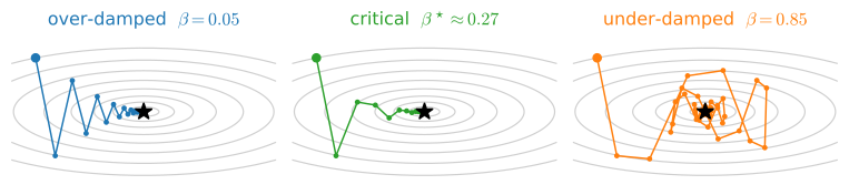
with momentum parameter \(\beta \in [0, 1)\); eliminating \(\mathbf{v}\) gives the equivalent form \(\mathbf{x}_{k+1} = \mathbf{x}_k - \eta \nabla f(\mathbf{x}_k) + \beta\,(\mathbf{x}_k - \mathbf{x}_{k-1})\). The update is named for the heavy-ball physical analogy, with friction parameter \(1 - \beta\). In each eigenmode of a quadratic, the update is a second-order linear recurrence (a damped oscillator), and \(\beta\) controls the damping. If damping is too strong, convergence along the low-curvature mode remains slow. If damping is too weak, the iterate oscillates around the minimum. Critical tuning gives the fastest decay in this quadratic model. Figure 26.1.3 shows all three regimes on the ill-conditioned valley.
26.1.4.2 The \(\sqrt{\kappa}\) Law
On quadratics, the effect of momentum can be computed exactly. Tuning both parameters optimally gives
\[ \eta^\star = \left(\frac{2}{\sqrt{\lambda_{\max}} + \sqrt{\lambda_{\min}}}\right)^{\!2}, \qquad \beta^\star = \left(\frac{\sqrt{\kappa} - 1}{\sqrt{\kappa} + 1}\right)^{\!2}, \]
heavy ball contracts every mode with asymptotic factor
\[ \rho_{\mathrm{HB}} = \frac{\sqrt{\kappa} - 1}{\sqrt{\kappa} + 1} \;\approx\; 1 - \frac{2}{\sqrt{\kappa}}, \tag{26.1.13}\]
so the iteration count drops from \(O(\kappa \log \tfrac1\varepsilon)\) to \(O(\sqrt{\kappa} \log \tfrac1\varepsilon)\) (Polyak 1964). The proof is a \(2 \times 2\) eigenvalue computation per mode (with the velocity, each mode’s state is two-dimensional, and the optimal tuning places every mode’s pair of eigenvalues on a circle of radius \(\sqrt{\beta^\star}\)), and Exercise 5 derives it. For \(\kappa = 10^4\), that is the difference between tens of thousands of iterations and hundreds.
The heavy-ball parameter formula and rate above are exact for quadratics; they do not constitute a guarantee for arbitrary strongly convex functions. Lessard et al. (2016) constructed a one-dimensional, smooth, strongly convex function on which heavy ball with the classical tuning does not converge at all: the iterates fall into a stable limit cycle. Momentum as deep learning uses it (Sutskever et al. 2013) is supported by the local quadratic model and broad empirical evidence, not by a global theorem for arbitrary strongly convex functions.
26.1.4.3 Nesterov’s Look-Ahead
There is a variant that does carry a global guarantee. Nesterov’s accelerated gradient (Nesterov 1983) evaluates the gradient not at the current point but at a look-ahead point displaced by the momentum:
\[ \mathbf{v}_{k+1} = \beta\, \mathbf{v}_k - \eta\, \nabla f(\mathbf{x}_k + \beta\, \mathbf{v}_k), \qquad \mathbf{x}_{k+1} = \mathbf{x}_k + \mathbf{v}_{k+1}. \tag{26.1.14}\]
The look-ahead gradient acts as a built-in correction: if the momentum is about to overshoot, the gradient at the look-ahead point already points back. For smooth convex \(f\) (with an appropriate \(\beta_k\) schedule) it achieves \(f(\mathbf{x}_k) - f^\star = O(1/k^2)\), beating plain gradient descent’s \(O(1/k)\) in Equation 26.1.10; for \(\mu\)-strongly convex \(f\) with \(\eta = 1/L\) and \(\beta = (\sqrt{\kappa}-1)/(\sqrt{\kappa}+1)\) it converges linearly with factor \(1 - 1/\sqrt{\kappa}\) (Nesterov 2018). These rates are optimal: the first-order oracle lower bound of Nemirovski and Yudin (1983) shows that no method forming its iterates from gradients and their linear combinations can improve on \(O(1/k^2)\), or beat \(\sqrt{\kappa}\) dependence, on the worst case over this problem class (see (Nesterov 2018) for the construction and proof). The worst-case construction uses a dimension that grows with the horizon, \(n \gtrsim 2k\), so the bound governs roughly the first \(n/2\) iterations. In a fixed dimension, sufficiently long runs can have better asymptotic behavior. For horizons much smaller than the parameter dimension, the dimensional restriction is inactive. The cell compares all three methods at a \(10^{-6}\) relative-error target as \(\kappa\) grows.
def iterations(lam, eta, beta=0.0, lookahead=False, tol=1e-6):
    """Steps until |x_k| <= tol |x_0| on f(x) = sum_i lam_i x_i^2 / 2."""
    x, v = np.array([1.0, 1.0]), np.zeros(2)
    n0 = np.linalg.norm(x)
    for k in range(1, 10**6):
        g = lam * (x + beta * v) if lookahead else lam * x
        v = beta * v - eta * g
        x = x + v
        if np.linalg.norm(x) <= tol * n0:
            return k

print('kappa      GD   heavy ball   Nesterov     GD/kappa   HB/sqrt(kappa)')
for kappa in [10.0, 100.0, 1000.0]:
    lam, sk = np.array([1.0, kappa]), np.sqrt(kappa)
    gd = iterations(lam, 2 / (1 + kappa))
    hb = iterations(lam, (2 / (1 + sk))**2, ((sk - 1) / (sk + 1))**2)
    na = iterations(lam, 1 / kappa, (sk - 1) / (sk + 1), lookahead=True)
    print(f'{kappa:5.0f} {gd:7d} {hb:9d} {na:10d}      '
          f'{gd / kappa:7.1f}     {hb / sk:7.1f}')
kappa GD heavy ball Nesterov GD/kappa HB/sqrt(kappa)
10 69 27 43 6.9 8.5
100 691 93 155 6.9 9.3
1000 6908 315 508 6.9 10.0The scaling columns show the predicted dependence. Gradient descent’s count divided by \(\kappa\) is approximately constant at \(6.9\) (exactly \(\tfrac12 \ln 10^6 \approx 6.9\), the constant our \((\kappa-1)/(\kappa+1) \approx 1 - 2/\kappa\) analysis predicts), so its cost is linear in \(\kappa\): \(6{,}908\) iterations at \(\kappa = 1000\). Heavy ball’s count grows like \(\sqrt{\kappa}\): \(315\) iterations at \(\kappa = 1000\), a \(22\times\) speedup. Its scaling column runs above the GD constant \(6.9\) because at the optimal tuning each extreme mode’s \(2 \times 2\) iteration matrix is defective, a repeated eigenvalue with only one eigenvector, the Jordan-block situation of Section 24.2.1.3.2; a polynomial factor \(k\rho^{k-1}\) therefore multiplies the geometric rate \(\rho^k\) and inflates the iteration count. Accordingly, the measured ratio increases across the table (\(8.5\), \(9.3\), \(10.0\)) toward \(\sqrt{\kappa}\)-consistent values rather than pinning at a constant. Nesterov’s iteration count lies between the two on this quadratic (\(508\) iterations): heavy ball is the quadratic specialist, while Nesterov’s slightly larger constant comes with a guarantee that extends to every smooth convex function. All three methods cost one gradient per iteration, so momentum’s speedup adds no per-step gradient cost. Momentum or exponential gradient averaging is consequently common in deep learning optimizers (Section 9.5).
26.1.5 Stochastic Gradients and Second-Order Tradeoffs
26.1.5.1 The Cost of Full Gradients
A training loss is an average over data,
\[ f(\mathbf{w}) = \frac{1}{N} \sum_{i=1}^N f_i(\mathbf{w}), \]
where \(f_i\) is the loss on example \(i\). The exact gradient \(\nabla f = \tfrac1N \sum_i \nabla f_i\) touches all \(N\) examples; at \(N \sim 10^9\), one gradient-descent step costs a full pass over the dataset. Stochastic gradient descent replaces the exact gradient with an estimate from a random minibatch \(B\) of \(b\) indices, drawn uniformly (for the analysis, with replacement):
\[ \hat{\mathbf{g}}_b = \frac{1}{b} \sum_{i \in B} \nabla f_i(\mathbf{w}), \qquad \mathbf{w}_{k+1} = \mathbf{w}_k - \eta_k\, \hat{\mathbf{g}}_b. \tag{26.1.15}\]
The estimate has two basic properties that recur in minibatch analyses.
Proposition (minibatch gradients: unbiased, variance \(\propto 1/b\)). Let \(\Sigma\) denote the covariance of a single uniformly drawn example gradient, \(\Sigma = \tfrac1N \sum_i \big(\nabla f_i - \nabla f\big)\big(\nabla f_i - \nabla f\big)^\top\) (all gradients at the current \(\mathbf{w}\)). Then
\[ \mathbb{E}\big[\hat{\mathbf{g}}_b\big] = \nabla f(\mathbf{w}), \qquad \mathbb{E}\big[\|\hat{\mathbf{g}}_b - \nabla f(\mathbf{w})\|^2\big] = \frac{\mathrm{tr}\, \Sigma}{b}. \tag{26.1.16}\]
Proof. Each index is uniform on \(\{1, \ldots, N\}\), so each term has expectation \(\tfrac1N \sum_i \nabla f_i = \nabla f\); by linearity so does the average. This equality depends on uniform sampling and on conditioning on the current iterate; biased sampling requires a correction. For the variance, the \(b\) draws are independent and identically distributed, so the covariance of their average is \(\Sigma / b\) (covariances of independent terms add, and the \(1/b\) outside enters squared). Taking the trace turns covariance into expected squared error. \(\blacksquare\)
The expected squared estimation error falls like \(1/b\), while its root-mean-square magnitude falls like \(1/\sqrt{b}\): increasing the batch computation by \(100\times\) reduces this magnitude by only \(10\times\). This scaling contributes to diminishing returns from very large batches (Exercise 7); the practical operating point also depends on parallel hardware and optimization dynamics. The cell verifies both claims on a hand-rolled logistic-regression problem, the toy we will keep for the rest of the section: \(n = 200\) points in five dimensions, labels flipped with logistic noise, plus a small \(\ell_2\) regularizer that makes the loss strongly convex.
rng = np.random.default_rng(42)
n, d = 200, 5
w_true = np.array([1.0, -2.0, 1.5, 0.0, 2.0])
X = rng.normal(size=(n, d))
y = np.where(rng.random(n) < 1 / (1 + np.exp(-X @ w_true)), 1.0, -1.0)
lam_reg = 0.1

def loss(w):
    return np.mean(np.log1p(np.exp(-y * (X @ w)))) + 0.5 * lam_reg * w @ w

def example_grads(w):                        # row i: gradient of example i's loss
    s = 1 / (1 + np.exp(y * (X @ w)))        # sigma(-y_i x_i^T w)
    return -(y * s)[:, None] * X + lam_reg * w

G = example_grads(np.zeros(d))
g_full = G.mean(axis=0)
tr_sigma = ((G - g_full)**2).sum(axis=1).mean()   # tr Sigma over the dataset
print(f'single-example gradient noise  tr Sigma = {tr_sigma:.4f}')
for b in [1, 4, 16, 64]:
    batches = rng.integers(0, n, size=(2000, b))  # 2000 minibatches per size
    err = ((G[batches].mean(axis=1) - g_full)**2).sum(axis=1).mean()
    print(f'b = {b:2d}:  measured E|g_hat - g|^2 = {err:.5f}   '
          f'predicted tr Sigma / b = {tr_sigma / b:.5f}')
single-example gradient noise tr Sigma = 1.1447
b = 1: measured E|g_hat - g|^2 = 1.15464 predicted tr Sigma / b = 1.14466
b = 4: measured E|g_hat - g|^2 = 0.28471 predicted tr Sigma / b = 0.28617
b = 16: measured E|g_hat - g|^2 = 0.07119 predicted tr Sigma / b = 0.07154
b = 64: measured E|g_hat - g|^2 = 0.01824 predicted tr Sigma / b = 0.01789At the initialization the single-example noise level is \(\mathrm{tr}\,\Sigma = 1.1447\), and the measured squared error of the minibatch gradient tracks the \(1/b\) prediction within Monte Carlo error at every batch size: \(1.155\) vs. \(1.145\) at \(b = 1\), down to \(0.0182\) vs. \(0.0179\) at \(b = 64\).
26.1.5.2 Stationary Error under Fixed-Step SGD
What does persistent gradient noise do to convergence? A one-dimensional strongly convex quadratic gives an exact recurrence. Model the update as \(x_{k+1} = x_k - \eta\,(\lambda x_k + \xi_k)\) with i.i.d. noise \(\mathbb{E}[\xi_k] = 0\), \(\mathbb{E}[\xi_k^2] = \sigma^2\). Squaring and taking expectations (the cross term vanishes by unbiasedness),
\[ \mathbb{E}\big[x_{k+1}^2\big] = (1 - \eta\lambda)^2\, \mathbb{E}\big[x_k^2\big] + \eta^2 \sigma^2, \]
a contraction plus a constant noise injection, whose fixed point is
\[ \mathbb{E}\big[x_\infty^2\big] = \frac{\eta^2 \sigma^2}{1 - (1 - \eta\lambda)^2} = \frac{\eta\, \sigma^2}{\lambda\, (2 - \eta\lambda)} \;\approx\; \frac{\eta\, \sigma^2}{2\lambda} \qquad (\eta \ll 1/\lambda). \tag{26.1.17}\]
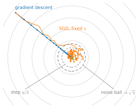
In this scalar quadratic model, fixed-step SGD does not converge to the minimizer; it converges to a stationary distribution whose iterates fluctuate inside a noise ball of squared radius proportional to \(\eta\,\sigma^2\), as in Figure 26.1.4. Far from the optimum the contraction term dominates and SGD makes GD-like linear progress; once the error reaches the ball, signal and noise balance, and subsequent iterates continue to fluctuate within the stationary distribution. The radius formula is a design guide: halving \(\eta\) halves the squared radius (and so does quadrupling \(b\), since \(\sigma^2 \mapsto \sigma^2/b\) by 2; step size and batch size are coupled parameters, the coupling behind the practical recipes of Section 9.4).
Under the persistent-noise assumptions of this model, convergence to the minimizer requires a decaying step: fast enough to control the noise, slowly enough to retain cumulative movement. The classical conditions of Robbins and Monro (1951) make both demands precise:
\[ \sum_{k} \eta_k = \infty, \qquad \sum_{k} \eta_k^2 < \infty. \tag{26.1.18}\]
These step-size conditions are only one part of a convergence theorem. With unbiased stochastic gradients, controlled second moments, a smooth strongly convex objective, and a suitable constant in \(\eta_k \propto 1/k\), SGD attains \(\mathbb{E}[f(\mathbf{w}_k)] - f^\star = O(1/k)\). For a convex but not strongly convex objective, appropriately scheduled SGD or averaged iterates attain the usual \(O(1/\sqrt{k})\) stochastic rate; Polyak–Ruppert averaging has sharper asymptotic conclusions under its own regularity conditions (Polyak and Juditsky 1992; Bottou 2010; Goodfellow et al. 2016). A condition on the constant is easy to miss: with \(\eta_k = c/k\), the \(O(1/k)\) guarantee requires \(c\) large enough relative to the curvature, \(c > 1/(2\mu)\); choose \(c\) too small and the rate degrades to \(O(k^{-2\mu c})\), arbitrarily slower than advertised, one reason practical schedules decay more gently than \(1/k\) (Bottou et al. 2018). Compare the deterministic linear rate Equation 26.1.11: noise changes the rate class, from geometric to polynomial. The cell shows both regimes on the logistic toy: fixed steps approach an \(\eta\)-proportional floor, whereas the decaying schedule continues toward zero.
w_star = np.zeros(d)
for _ in range(4000):                         # full-batch reference optimum
    w_star = w_star - 0.5 * example_grads(w_star).mean(axis=0)
f_star = loss(w_star)

def sgd(schedule, steps=4000, b=8, seed=1):
    rg = np.random.default_rng(seed)
    w, gaps = np.zeros(d), []
    for k in range(steps):
        idx = rg.integers(0, n, size=b)
        s = 1 / (1 + np.exp(y[idx] * (X[idx] @ w)))
        g = (-(y[idx] * s)[:, None] * X[idx]).mean(axis=0) + lam_reg * w
        w = w - schedule(k) * g
        gaps.append(loss(w) - f_star)
    return np.array(gaps)

gap_fix = sgd(lambda k: 0.8)
gap_half = sgd(lambda k: 0.4)
gap_dec = sgd(lambda k: 0.8 / (1 + k / 100))
print(f'fixed eta = 0.8:     mean gap, last 1000 steps = {gap_fix[-1000:].mean():.2e}')
print(f'fixed eta = 0.4:     mean gap, last 1000 steps = {gap_half[-1000:].mean():.2e}')
print(f'decay 0.8/(1+k/100): mean gap, last 1000 steps = {gap_dec[-1000:].mean():.2e}')
d2l.plot(np.arange(1, 4001), [gap_fix, gap_dec], 'step k', 'optimality gap',
         xscale='log', yscale='log',
legend=['fixed eta = 0.8', 'decay 0.8/(1+k/100)'])fixed eta = 0.8: mean gap, last 1000 steps = 2.34e-02
fixed eta = 0.4: mean gap, last 1000 steps = 1.08e-02
decay 0.8/(1+k/100): mean gap, last 1000 steps = 5.67e-04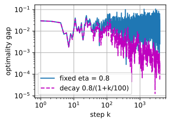
fixed eta = 0.8:     mean gap, last 1000 steps = 2.34e-02
fixed eta = 0.4:     mean gap, last 1000 steps = 1.08e-02
decay 0.8/(1+k/100): mean gap, last 1000 steps = 5.67e-04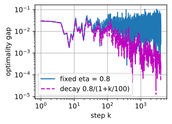
fixed eta = 0.8:     mean gap, last 1000 steps = 2.34e-02
fixed eta = 0.4:     mean gap, last 1000 steps = 1.08e-02
decay 0.8/(1+k/100): mean gap, last 1000 steps = 5.67e-04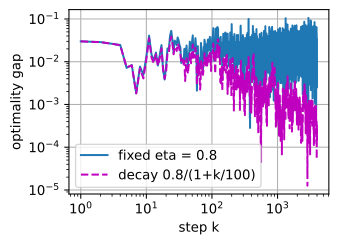
fixed eta = 0.8:     mean gap, last 1000 steps = 2.34e-02
fixed eta = 0.4:     mean gap, last 1000 steps = 1.08e-02
decay 0.8/(1+k/100): mean gap, last 1000 steps = 5.67e-04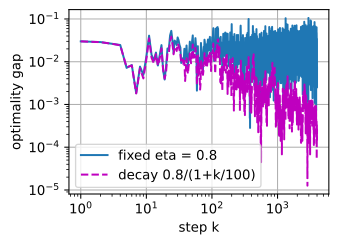
The measurements agree with the theoretical predictions. Fixed \(\eta = 0.8\) stalls at an average gap of \(2.3 \times 10^{-2}\); halving the step to \(0.4\) halves the floor to \(1.1 \times 10^{-2}\): the linear-in-\(\eta\) noise ball of Equation 26.1.17, measured. The \(1/k\) schedule is at \(5.7 \times 10^{-4}\) after the same \(4000\) steps and still descending as a power law, the straight line on the log-log plot: its early large steps cross the valley, and its late small steps shrink the ball. Modern schedules (step decay, cosine, and warmup; Section 9.3 and Section 9.4) manage this tradeoff empirically on losses that are neither convex nor stationary. Warmup starts with a small \(\eta\) and ramps it upward. It can reduce early instability while gradient statistics and local curvature are changing rapidly, but the quadratic analysis does not establish a universal warmup rule for neural networks. Schedules and warmup are discussed in Section 26.2.
The main curvature-based choices differ in what they store and how they control a proposed step:
| Method | Curvature representation | Storage | Step computation and safeguard |
|---|---|---|---|
| Gradient descent or momentum | none | \(O(d)\) | gradient step; fixed schedule or line search |
| Newton | dense Hessian | \(O(d^2)\) | dense linear solve; damping or trust region away from a local minimum |
| BFGS | dense inverse-Hessian estimate | \(O(d^2)\) | matrix–vector product; usually a Wolfe line search |
| L-BFGS | \(m\) recent secant pairs | \(O(md)\) | two-loop recursion and line search |
| Trust-region Newton/CG | Hessian or Hessian–vector products | implementation-dependent | approximate constrained quadratic solve; acceptance by model agreement |
26.1.5.3 Newton’s Method and Its Computational Cost
The preceding first-order analysis treats curvature as a restriction on step size and iteration count. Newton’s method instead uses curvature to choose the step. Minimize the local quadratic model exactly (the \(n\)-dimensional version of Section 25.1.4.4) by solving for its stationary point:
\[ \mathbf{x}_{k+1} = \mathbf{x}_k - \big(\nabla^2 f(\mathbf{x}_k)\big)^{-1} \nabla f(\mathbf{x}_k). \tag{26.1.19}\]
On a quadratic \(f(\mathbf{x}) = \tfrac12 \mathbf{x}^\top A \mathbf{x}\), the model is the function, so one step lands exactly on the minimizer: \(\mathbf{x}_1 = \mathbf{x}_0 - A^{-1} A \mathbf{x}_0 = \mathbf{0}\), for every \(\kappa\). The quadratic Newton step is independent of the condition number because the method is affine-invariant: rescale or shear the coordinates, \(\mathbf{x} = T\mathbf{y}\), and Newton’s iterates transform equivariantly through \(T\) (Exercise 8): coordinate rescaling does not change Newton’s iteration count on this quadratic, while gradient descent’s behavior changes with every reparametrization. Started close enough to a minimizer whose Hessian is positive definite and Lipschitz continuous in a neighborhood, Newton converges quadratically, \(\|\mathbf{x}_{k+1} - \mathbf{x}^\star\| \le C\,\|\mathbf{x}_k - \mathbf{x}^\star\|^2\) (Theorem 3.5 of Nocedal and Wright (2006)): the local error is squared at each iteration, which approximately doubles the number of correct digits. The cell shows both facts: a one-step solve of the \(\kappa = 100\) quadratic that costs gradient descent \(691\) iterations, and the doubling-digits signature on our logistic toy.
A2 = np.diag([1.0, 100.0])                    # kappa = 100
x = np.array([1.0, 1.0])
x_new = x - np.linalg.solve(A2, A2 @ x)       # one Newton step
rate = (100 - 1) / (100 + 1)
print(f'Newton on the quadratic: |x_1| = {np.linalg.norm(x_new):.1e} after one step')
print(f'GD with the optimal step contracts by {rate:.4f} per step; it needs '
      f'{int(np.ceil(np.log(1e-6) / np.log(rate)))} steps for |x_k| <= 1e-6')
w = np.zeros(d)                               # Newton on the logistic loss
for it in range(6):
    s = 1 / (1 + np.exp(y * (X @ w)))
    g = example_grads(w).mean(axis=0)
    H = (X * (s * (1 - s))[:, None]).T @ X / n + lam_reg * np.eye(d)
    w = w - np.linalg.solve(H, g)
    print(f'Newton iteration {it + 1}:  |grad| = {np.linalg.norm(g):.1e}')
print('agrees with the SGD section optimum:', bool(np.allclose(w, w_star, atol=1e-8)))
Newton on the quadratic: |x_1| = 0.0e+00 after one step
GD with the optimal step contracts by 0.9802 per step; it needs 691 steps for |x_k| <= 1e-6
Newton iteration 1: |grad| = 2.8e-01
Newton iteration 2: |grad| = 3.2e-02
Newton iteration 3: |grad| = 1.1e-03
Newton iteration 4: |grad| = 1.2e-06
Newton iteration 5: |grad| = 1.6e-12
Newton iteration 6: |grad| = 3.1e-17
agrees with the SGD section optimum: TrueThe gradient norms fall as \(2.8 \times 10^{-1}\), \(3.2 \times 10^{-2}\), \(1.1 \times 10^{-3}\), \(1.2 \times 10^{-6}\), \(1.6 \times 10^{-12}\) (the exponent roughly doubling each time, consistent with quadratic convergence), and six iterations reproduce, to \(10^{-8}\), the optimum that \(4000\) full-batch gradient steps computed in the previous cell.
Dense Newton steps do not scale to modern parameter counts: the Hessian has \(d^2\) entries and a generic factorization costs \(O(d^3)\). The objection is structural as well: away from a minimum the Hessian of a nonconvex loss is typically indefinite, and the Newton direction can point toward a saddle unless safeguarded, because it seeks a stationary point of the model, any stationary point. Large-scale methods therefore use cheaper curvature surrogates. L-BFGS rebuilds a low-rank curvature estimate from recent gradient differences with \(O(d)\) memory (Liu and Nocedal 1989), and the adaptive family (AdaGrad (Duchi et al. 2011), RMSProp (Tieleman and Hinton 2012), Adam (Kingma and Ba 2015)) maintains a diagonal preconditioner, a per-coordinate learning rate (Section 9.6). Between the diagonal and the full matrix sit the structured preconditioners that 2020s practice has made mainstream, K-FAC (Martens and Grosse 2015), Shampoo (Gupta et al. 2018), and Muon (Jordan et al. 2024), which exploit the fact that a network’s parameters come in matrices rather than one long vector. First-order methods with curvature surrogates, fed by minibatch gradients: that is the compromise this section has been deriving, and deep-learning libraries implement variants of this compromise. The mathematics of this family is the subject of Section 26.2.
26.1.5.4 Quasi-Newton Methods: Curvature from Secants
Newton uses the Hessian as a local map from a step to a gradient change. A quasi-Newton method infers that map from differences it has already observed. After moving by
\[ \mathbf s_k=\mathbf x_{k+1}-\mathbf x_k, \qquad \mathbf y_k=\nabla f(\mathbf x_{k+1})-\nabla f(\mathbf x_k), \]
an inverse-Hessian approximation \(H_{k+1}\) should satisfy the secant equation \(H_{k+1}\mathbf y_k=\mathbf s_k\). One vector equation cannot determine a whole matrix, so BFGS chooses the symmetric rank-two update closest to the previous approximation in a suitable matrix metric:
\[ H_{k+1} =(I-\rho_k\mathbf s_k\mathbf y_k^\top)H_k (I-\rho_k\mathbf y_k\mathbf s_k^\top) +\rho_k\mathbf s_k\mathbf s_k^\top, \qquad \rho_k=(\mathbf y_k^\top\mathbf s_k)^{-1}. \tag{26.1.20}\]
When \(H_k\) is positive definite and the curvature condition \(\mathbf y_k^\top\mathbf s_k>0\) holds, the update remains positive definite, so \(-H_k\nabla f\) is a descent direction. A Wolfe line search is commonly used because its conditions imply this positive-curvature test on a smooth objective. On a strongly convex quadratic with exact line searches, BFGS recovers the solution in at most \(d\) iterations in exact arithmetic: each secant pair identifies another curvature direction.
rng = np.random.default_rng(9)
d_bfgs = 6
Q, _ = np.linalg.qr(rng.standard_normal((d_bfgs, d_bfgs)))
A_bfgs = Q @ np.diag(np.geomspace(1., 1000., d_bfgs)) @ Q.T
b_bfgs = rng.standard_normal(d_bfgs)
x_star_bfgs = np.linalg.solve(A_bfgs, b_bfgs)
x_bfgs, H_bfgs = np.zeros(d_bfgs), np.eye(d_bfgs)
x_gd = np.zeros(d_bfgs)
eta_gd = 2 / (1 + 1000)                       # optimal fixed quadratic step
dist_bfgs, dist_gd = [], []
for k in range(d_bfgs):
    g = A_bfgs @ x_bfgs - b_bfgs
    p_bfgs = -H_bfgs @ g
    alpha = -(g @ p_bfgs) / (p_bfgs @ A_bfgs @ p_bfgs)  # exact line search
    step = alpha * p_bfgs
    y_diff = A_bfgs @ step
    rho = 1.0 / (y_diff @ step)
    V = np.eye(d_bfgs) - rho * np.outer(step, y_diff)
    H_bfgs = V @ H_bfgs @ V.T + rho * np.outer(step, step)
    x_bfgs += step
    x_gd -= eta_gd * (A_bfgs @ x_gd - b_bfgs)
    dist_bfgs.append(np.linalg.norm(x_bfgs - x_star_bfgs))
    dist_gd.append(np.linalg.norm(x_gd - x_star_bfgs))
d2l.plot(np.arange(1, d_bfgs + 1), [dist_gd, dist_bfgs],
         'iteration', 'distance to optimum',
         legend=['gradient descent', 'BFGS'], yscale='log')
print(f'after d = {d_bfgs} steps: BFGS {dist_bfgs[-1]:.2e}, '
f'GD {dist_gd[-1]:.2e}')after d = 6 steps: BFGS 1.05e-14, GD 7.94e-01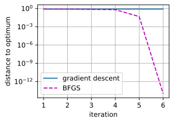
after d = 6 steps: BFGS 1.05e-14, GD 7.94e-01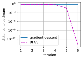
after d = 6 steps: BFGS 1.05e-14, GD 7.94e-01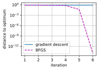
after d = 6 steps: BFGS 1.05e-14, GD 7.94e-01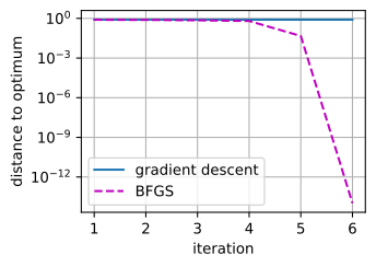
The finite-termination property is an ideal quadratic benchmark, not a promise for a neural loss. In general the line search is inexact, curvature changes, and stochastic gradients corrupt \(\mathbf y_k\). Full BFGS also stores a dense \(d\times d\) matrix. L-BFGS keeps only the most recent \(m\) secant pairs and applies the implied inverse by a two-loop recursion, reducing storage and work to \(O(md)\). This makes it attractive for deterministic medium-scale problems and full-batch fine-tuning, but less natural when fresh minibatch noise makes gradient differences unreliable.
26.1.5.5 Trust Regions and Model Agreement
Line search first chooses a direction and then decides how far to travel along it. A trust-region method instead constrains the quadratic-model step to a region in which the model is expected to be accurate:
\[ \min_{\|\mathbf p\|\le\Delta_k} m_k(\mathbf p) =f(\mathbf x_k)+\nabla f(\mathbf x_k)^\top\mathbf p +\tfrac12\mathbf p^\top B_k\mathbf p. \tag{26.1.21}\]
The radius \(\Delta_k\) prevents an inaccurate local model from making an arbitrarily large proposal and makes the subproblem bounded even when \(B_k\) has a negative eigenvalue. After approximately solving the subproblem, compare actual with predicted improvement,
\[ r_k= \frac{f(\mathbf x_k)-f(\mathbf x_k+\mathbf p_k)} {m_k(\mathbf 0)-m_k(\mathbf p_k)}. \tag{26.1.22}\]
A ratio near one says the model predicted the step well, so accept it and possibly enlarge the radius. A small or negative ratio rejects the step and shrinks the radius. Thus measured agreement between the objective and model determines the radius. Exact trust-region solves are unnecessary: the dogleg method combines steepest descent with Newton on positive-definite models, while truncated conjugate gradient stops at the boundary or upon finding negative curvature using only Hessian–vector products (Section 25.3).
Trust regions and quasi-Newton updates solve complementary problems. BFGS asks how to estimate curvature without forming a Hessian; a trust region asks how to safeguard whichever model we have. Neither displaces SGD for enormous noisy objectives, but both are important for smaller deterministic models, inner optimization problems, and understanding what “second order” means beyond explicitly inverting a Hessian.
26.1.6 Summary
- A direction \(\mathbf{d}\) is a descent direction iff \(\nabla f^\top \mathbf{d} < 0\); among unit directions the steepest is \(-\nabla f / \|\nabla f\|\) by Cauchy–Schwarz. Descent directions form a half-space; gradient descent chooses the steepest local direction.
- \(L\)-smoothness gives a quadratic upper bound and yields the descent lemma: progress \(\eta(1 - L\eta/2)\,\|\nabla f\|^2\) per step, positive for \(\eta < 2/L\), best guaranteed at \(\eta = 1/L\). Telescoping it gives \(\min_k \|\nabla f(\mathbf{x}_k)\|^2 \le 2L(f(\mathbf{x}_0) - f^\star)/K\): stationarity at rate \(O(1/K)\) with no convexity, a useful smooth-model benchmark for deep networks rather than a literal guarantee for nonsmooth architectures or trajectories without a finite smoothness bound. Backtracking line search achieves a step within a constant of \(1/L\) without knowing \(L\).
- On a quadratic, GD decouples into per-mode factors \(1 - \eta\lambda_i\): stability demands \(\eta < 2/L\), the optimal step \(\eta^\star = 2/(\lambda_{\min} + \lambda_{\max})\) contracts by exactly \((\kappa - 1)/(\kappa + 1)\), and the cost of gradient descent is linear in \(\kappa\). Some neural-network experiments exhibit an edge-of-stability regime in which measured sharpness tracks the local \(2/\eta\) threshold.
- Convexity upgrades stationarity to global optimality: \(O(1/k)\) values for smooth convex, linear rate \((1 - 1/\kappa)^k\) for strongly convex; stated here, proved in Section 26.3.
- Momentum turns each mode into a damped oscillator and improves the rate to \((\sqrt{\kappa} - 1)/(\sqrt{\kappa} + 1)\) on quadratics; Nesterov’s look-ahead achieves \(O(1/k^2)\) and \(\sqrt{\kappa}\) dependence with a global guarantee, and these rates are optimal for first-order methods. Heavy ball’s \(\sqrt{\kappa}\) is quadratic-only: it can cycle on general strongly convex functions.
- Minibatch gradients are unbiased with variance \(\mathrm{tr}\,\Sigma / b\). On the scalar quadratic model, fixed-step SGD has a noise ball of squared radius \(\approx \eta\sigma^2/(2\lambda)\). Under the usual stochastic approximation assumptions, Robbins–Monro decay (\(\sum \eta_k = \infty\), \(\sum \eta_k^2 < \infty\)) permits convergence to the optimum.
- In exact arithmetic, Newton’s method solves a positive-definite quadratic in one step regardless of \(\kappa\). Near a regular minimizer it is locally quadratically convergent, but a dense implementation costs \(O(d^2)\) memory and \(O(d^3)\) time per step. BFGS learns an inverse-Hessian approximation from secant pairs; L-BFGS stores only a short history. Trust-region methods bound the quadratic model’s step and use actual-versus-predicted improvement to adjust that bound, making curvature useful without trusting it globally.
26.1.7 Exercises
Prove the descent lemma Equation 26.1.5 from \(L\)-smoothness without looking, and show that \(\eta = 1/L\) maximizes the guaranteed per-step decrease \(\eta(1 - L\eta/2)\,\|\nabla f\|^2\). What goes wrong in the bound (and in practice) at \(\eta = 2/L\) exactly?
Show that \(\mathbf{d} = -B\,\nabla f(\mathbf{x})\) is a descent direction for every positive definite matrix \(B\). Then find the steepest descent direction when length is measured by the norm \(\|\mathbf{d}\|_A = \sqrt{\mathbf{d}^\top A \mathbf{d}}\) for positive definite \(A\), and recognize the answer as a preconditioned gradient: with \(A = \nabla^2 f\), as Newton’s direction. (Hint: substitute \(\mathbf{u} = A^{1/2}\mathbf{d}\) and reuse Cauchy–Schwarz.)
Derive the optimal step \(\eta^\star = 2/(\lambda_{\min} + \lambda_{\max})\) by minimizing \(\max_i |1 - \eta\lambda_i|\), confirm the contraction factor \((\kappa - 1)/(\kappa + 1)\), and explain geometrically why \(\kappa \to 1\) gives convergence in a single step.
On \(f(\mathbf{x}) = \tfrac12(\lambda_1 x_1^2 + \lambda_2 x_2^2)\) with \(\lambda_1 = 1\), \(\lambda_2 = 10\), choose a step size with \(2/\lambda_2 < \eta < 2/\lambda_1\) and run twenty iterations from \((1, 1)\). Verify that one coordinate converges while the other diverges, and reconcile this with the spectral-radius criterion of
Write heavy ball Equation 26.1.12 on the one-dimensional quadratic \(f(x) = \tfrac{\lambda}{2} x^2\) as a linear map of the state \((x_k, x_{k-1})\), and compute the eigenvalues of its \(2 \times 2\) iteration matrix. Show that for \(\beta \ge (1 - \sqrt{\eta\lambda})^2\) the eigenvalues are complex with modulus \(\sqrt{\beta}\) (independent of \(\lambda\)), and conclude that the tuning Equation 26.1.13 contracts every mode of a quadratic at rate \((\sqrt{\kappa}-1)/(\sqrt{\kappa}+1)\).
Prove the unbiasedness and \(1/b\) variance of
- Now suppose the minibatch is drawn without replacement. Show the estimate is still unbiased, and that its covariance acquires the finite-population factor \(\tfrac{N - b}{N - 1}\), so sampling without replacement is (slightly) better, and exact at \(b = N\).
Use Equation 26.1.17 to argue that no constant step size can converge to the minimizer while the gradient noise at the optimum is nonzero. Then study the tradeoff: combining 2 and Equation 26.1.17, the noise-ball radius scales like \(\eta\sigma^2 / b\). Doubling \(b\) doubles per-step compute and halves the ball; halving \(\eta\) halves the ball but slows the transient. Discuss when large batches are worth it (hint: wall-clock time under data parallelism vs. total FLOPs), and check the prediction against the schedule-comparison experiment above, where halving \(\eta\) halved the measured floor.
Newton: show that on any strictly convex quadratic, the step Equation 26.1.19 reaches the minimizer in one iteration regardless of \(\kappa\). Show affine invariance: if \(g(\mathbf{y}) = f(T\mathbf{y})\) for invertible \(T\), Newton iterates for \(g\) satisfy \(\mathbf{y}_k = T^{-1}\mathbf{x}_k\) where \(\mathbf{x}_k\) are Newton iterates for \(f\) (while gradient descent has no such property). Finally, compare the \(O(d^2)\) storage and \(O(d^3)\) factorization of dense Newton with a truncated-CG step using \(m\) Hessian–vector products and \(O(d)\) working memory. State which structure makes the latter feasible at large \(d\) and which Newton safeguards it still requires on a nonconvex objective.
Implicit bias. Let \(X \in \mathbb{R}^{n \times d}\) with \(n < d\) and full row rank, and minimize the underdetermined least-squares loss \(f(\mathbf{w}) = \tfrac12\|X\mathbf{w} - \mathbf{y}\|^2\), which has infinitely many global minimizers. Show that every gradient (hence, started from \(\mathbf{w}_0 = \mathbf{0}\), every GD iterate) lies in the row space of \(X\); show that the unique minimizer within the row space is the minimum-norm interpolator \(\mathbf{w}^\dagger = X^\top (X X^\top)^{-1} \mathbf{y}\); and conclude that gradient descent with any fixed step size \(0 < \eta < 2/\lambda_{\max}(X^\top X)\) converges to it. Moral: when minimizers are plentiful, the optimizer, not the loss, chooses among them, a theme that returns for deep networks in Section 26.3. (This exercise is deliberately pencil-and-paper; its numerical companion, observing convergence to \(\mathbf{w}^\dagger\), is Exercise 8 of Section 26.3.)
BFGS and the secant equation. Verify directly that the update Equation 26.1.20 is symmetric and satisfies \(H_{k+1}\mathbf y_k=\mathbf s_k\). Show that it remains positive definite when \(H_k\succ0\) and \(\mathbf y_k^\top\mathbf s_k>0\).
Trust-region acceptance. For \(f(x)=\tfrac14x^4-\tfrac12x^2\) at \(x=0.2\), form the quadratic Taylor model. Solve the one-dimensional trust-region subproblem for several radii \(\Delta\), compute Equation 26.1.22, and determine which proposals should be accepted. What goes wrong with the unrestricted Newton step at this point?
26.1.8 Discussions
This section is the rate-and-condition-number justification for the main book’s optimization chapter: Section 9.2 implements gradient descent, Section 9.3 and Section 9.4 develop its stochastic practice, and Section 9.5 and Section 9.6 introduce momentum and adaptive methods; the descent lemma, the \(\kappa\) and \(\sqrt{\kappa}\) laws, the \(1/b\) variance, and the noise ball proved here are the reasons those recipes work. Within this part, the convexity that upgrades stationarity to optimality is developed next in Section 26.3, constraints and duality follow in Section 26.4, and the condition number returns in its numerical role, measuring error amplification, in Section 26.5.