4.1  Multilayer Perceptrons

Softmax regression maps its inputs to class scores with a single affine transformation. This makes the model easy to optimize but restricts its decision boundaries. Multilayer perceptrons add one or more hidden layers and nonlinear activation functions, allowing the model to represent nonlinear relations while retaining the same data, loss, and optimization procedure.

%matplotlib inline
from d2l import torch as d2l
import torch
import numpy as onp
%matplotlib inline
from d2l import tensorflow as d2l
import tensorflow as tf
import numpy as onp
%matplotlib inline
from d2l import jax as d2l
import jax
from jax import numpy as jnp
from jax import grad, vmap
import numpy as onp
%matplotlib inline
from d2l import mxnet as d2l
from mxnet import autograd, np, npx
import numpy as onp
npx.set_np()
4.1.1 Hidden Layers

We described affine transformations in Section 2.1.1.1 as linear transformations with added bias. To begin, recall the model architecture corresponding to our softmax regression example, illustrated in Figure 3.1.1. This model maps inputs directly to outputs via a single affine transformation, followed by a softmax operation. If our labels truly were related to the input data by a simple affine transformation, then this approach would be sufficient. However, linearity (in affine transformations) is a strong assumption.

4.1.1.1 Limitations of Linear Models

For example, linearity implies the weaker assumption of monotonicity, i.e., that any increase in our feature must either always cause an increase in our model’s output (if the corresponding weight is positive), or always cause a decrease in our model’s output (if the corresponding weight is negative). Sometimes that makes sense. For example, if we were trying to predict whether an individual will repay a loan, we might reasonably assume that all other things being equal, an applicant with a higher income would always be more likely to repay than one with a lower income. While monotonic, this relationship likely is not linearly associated with the probability of repayment. An increase in income from $0 to $50,000 likely corresponds to a bigger increase in likelihood of repayment than an increase from $1 million to $1.05 million. One way to handle this might be to postprocess our outcome such that linearity becomes more plausible, by passing the outcome through the logistic function (i.e., modeling the log-odds linearly).

Note that we can easily come up with examples that violate monotonicity. Consider predicting health risk from body temperature. For individuals with a normal body temperature above 37°C (98.6°F), higher temperatures indicate greater risk. Below 37°C, however, lower temperatures also indicate greater risk. Again, we might resolve the problem with some clever preprocessing, such as using the distance from 37°C as a feature.

But what about classifying images of cats and dogs? Should increasing the intensity of the pixel at location (13, 17) always increase (or always decrease) the likelihood that the image depicts a dog? Reliance on a linear model corresponds to the implicit assumption that the only requirement for differentiating cats and dogs is to assess the brightness of individual pixels. This approach fails because transformations such as intensity inversion can preserve the category while changing every pixel value.

Unlike the preceding scalar examples, this problem has no evident fixed preprocessing solution because the significance of a pixel depends on its context, including the values of surrounding pixels. A representation that captures the relevant feature interactions might make a linear predictor suitable, but constructing such a representation manually is generally impractical. With deep neural networks, we use observational data to jointly learn both a representation via hidden layers and a linear predictor that acts upon that representation.

This problem of nonlinearity has been studied for at least a century (Fisher 1925). For instance, decision trees in their most basic form use a sequence of binary decisions to decide upon class membership (Quinlan 1993). Likewise, kernel methods have been used for many decades to model nonlinear dependencies (Aronszajn 1950), including nonparametric spline models (Wahba 1990). Biological neural systems also organize neurons in successive connections (Ramón y Cajal and Azoulay 1894), motivating models built from sequences of simple transformations.

4.1.1.2 Incorporating Hidden Layers

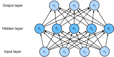
We can overcome the limitations of linear models by incorporating one or more hidden layers. The easiest way to do this is to stack many fully connected layers on top of one another. Each layer feeds into the layer above it, until we generate outputs. We can think of the first \(L-1\) layers as our representation and the final layer as our linear predictor. This architecture is commonly called a multilayer perceptron, often abbreviated as MLP (Figure 4.1.1).

Figure 4.1.1: An MLP with a hidden layer of five hidden units.

This MLP has four inputs, three outputs, and its hidden layer contains five hidden units. Since the input layer does not involve any calculations, producing outputs with this network requires implementing the computations for both the hidden and output layers; thus, the number of layers in this MLP is two. Note that both layers are fully connected. Every input influences every neuron in the hidden layer, and each of these in turn influences every neuron in the output layer. Alas, we are not quite done yet.

4.1.1.3 From Linear to Nonlinear

As before, we denote by the matrix \(\mathbf{X} \in \mathbb{R}^{n \times d}\) a minibatch of \(n\) examples where each example has \(d\) inputs (features). For a one-hidden-layer MLP whose hidden layer has \(h\) hidden units, we denote by \(\mathbf{H} \in \mathbb{R}^{n \times h}\) the outputs of the hidden layer, which are hidden representations. Since the hidden and output layers are both fully connected, we have hidden-layer weights \(\mathbf{W}^{(1)} \in \mathbb{R}^{d \times h}\) and biases \(\mathbf{b}^{(1)} \in \mathbb{R}^{1 \times h}\) and output-layer weights \(\mathbf{W}^{(2)} \in \mathbb{R}^{h \times q}\) and biases \(\mathbf{b}^{(2)} \in \mathbb{R}^{1 \times q}\). This allows us to calculate the outputs \(\mathbf{O} \in \mathbb{R}^{n \times q}\) of the one-hidden-layer MLP as follows:

\[ \begin{aligned} \mathbf{H} & = \mathbf{X} \mathbf{W}^{(1)} + \mathbf{b}^{(1)}, \\ \mathbf{O} & = \mathbf{H}\mathbf{W}^{(2)} + \mathbf{b}^{(2)}. \end{aligned} \]

Without a nonlinearity, the additional layer does not enlarge the represented function class. The hidden units are affine functions of the inputs, and the outputs are affine functions of those hidden units. A composition of affine maps is again affine, which the original linear model could already represent.

To verify this claim, substitute the hidden-layer expression into the output layer: yielding an equivalent single-layer model with parameters \(\mathbf{W} = \mathbf{W}^{(1)}\mathbf{W}^{(2)}\) and \(\mathbf{b} = \mathbf{b}^{(1)} \mathbf{W}^{(2)} + \mathbf{b}^{(2)}\):

\[ \mathbf{O} = (\mathbf{X} \mathbf{W}^{(1)} + \mathbf{b}^{(1)})\mathbf{W}^{(2)} + \mathbf{b}^{(2)} = \mathbf{X} \mathbf{W}^{(1)}\mathbf{W}^{(2)} + \mathbf{b}^{(1)} \mathbf{W}^{(2)} + \mathbf{b}^{(2)} = \mathbf{X} \mathbf{W} + \mathbf{b}. \]

In order to realize the potential of multilayer architectures, we need one more key ingredient: a nonlinear activation function \(\sigma\) to be applied to each hidden unit following the affine transformation. For instance, a popular choice is the ReLU (rectified linear unit) activation function (Nair and Hinton 2010), operating on its arguments elementwise. The outputs of activation functions \(\sigma(\cdot)\) are called activations. In general, with activation functions in place, it is no longer possible to collapse our MLP into a linear model:

\[ \begin{aligned} \mathbf{H} & = \sigma(\mathbf{X} \mathbf{W}^{(1)} + \mathbf{b}^{(1)}), \\ \mathbf{O} & = \mathbf{H}\mathbf{W}^{(2)} + \mathbf{b}^{(2)}.\\ \end{aligned} \]

Since each row in \(\mathbf{X}\) corresponds to an example in the minibatch, with some abuse of notation, we define the nonlinearity \(\sigma\) to apply to its inputs in a rowwise fashion, i.e., one example at a time. Note that we used the same notation for softmax when we denoted a rowwise operation in Section 3.1.2.1. Quite frequently the activation functions we use apply elementwise, a special case of rowwise. That means that after computing the linear portion of the layer, we can calculate each activation without looking at the values taken by the other hidden units.

To build more general MLPs, we can continue stacking such hidden layers, e.g., \(\mathbf{H}^{(1)} = \sigma_1(\mathbf{X} \mathbf{W}^{(1)} + \mathbf{b}^{(1)})\) and \(\mathbf{H}^{(2)} = \sigma_2(\mathbf{H}^{(1)} \mathbf{W}^{(2)} + \mathbf{b}^{(2)})\), one atop another, yielding ever more expressive models.

4.1.1.4 A Concrete Win: XOR

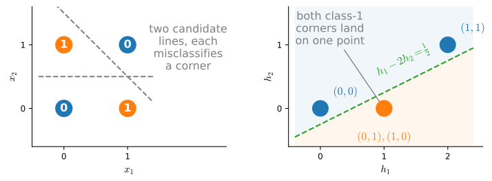
The collapse argument above establishes the limitation of a hidden layer without a nonlinearity. The smallest problem that demonstrates the effect of adding a nonlinearity is the exclusive-or (XOR) function. Place four points at the corners of the unit square and label each by whether its two coordinates differ: \((0,0)\) and \((1,1)\) get label \(0\), while \((0,1)\) and \((1,0)\) get label \(1\). As Figure 4.1.2 shows on the left, the two classes sit on opposite diagonals, so no straight line can put one class on each side. No linear classifier can solve this problem, regardless of how we choose its weights.

Figure 4.1.2: XOR is not linearly separable, but one ReLU hidden layer makes it so. Left: the four corners of the unit square, coloured by the XOR label (the digit on each marker); the two classes lie on opposite diagonals, so any line misclassifies a corner. Right: the same four points after the hidden map \(\mathbf{h} = \operatorname{ReLU}(\mathbf{x}\mathbf{W}^{(1)} + \mathbf{b}^{(1)})\) with \(\mathbf{W}^{(1)} = \left(\begin{smallmatrix}1 & 1\\ 1 & 1\end{smallmatrix}\right)\) and \(\mathbf{b}^{(1)} = (0, -1)\). The two class-1 corners are folded onto the same point \((1,0)\), and the cloud becomes linearly separable: the output neuron \(h_1 - 2h_2\) now realizes XOR.

A hidden layer with two ReLU units solves the problem by re-representing the inputs so that the two class-1 corners coincide in the hidden space. The classic choice (see Goodfellow et al. (2016), Chapter 6) uses

\[\mathbf{W}^{(1)} = \begin{pmatrix} 1 & 1 \\ 1 & 1 \end{pmatrix}, \quad \mathbf{b}^{(1)} = \begin{pmatrix} 0 & -1 \end{pmatrix}, \quad \mathbf{w}^{(2)} = \begin{pmatrix} 1 \\ -2 \end{pmatrix}, \quad b^{(2)} = 0, \tag{4.1.1}\]

with a ReLU on the hidden layer. The first hidden unit fires for any “active” input; the second only fires when both coordinates are on, and subtracting twice the second unit cancels the lone case the first unit gets wrong. The right panel of Figure 4.1.2 plots the hidden representation: the two label-1 corners land on top of each other at \((1,0)\), after which a single line separates the classes. We verify that this hand-built network computes XOR exactly on all four inputs.

X = onp.array([[0., 0.], [0., 1.], [1., 0.], [1., 1.]])
W1 = onp.array([[1., 1.], [1., 1.]])
b1 = onp.array([0., -1.])
w2 = onp.array([[1.], [-2.]])
H = onp.maximum(X @ W1 + b1, 0)
O = (H @ w2).squeeze()
onp.column_stack([X, (O > 0.5).astype(float)])
array([[0., 0., 0.],
       [0., 1., 1.],
       [1., 0., 1.],
       [1., 1., 0.]])

The third column is exactly the XOR of the first two. We constructed the weights here, but the whole point of the rest of this book is that optimization can discover such representations from data. The same principle generalizes: stacked nonlinear hidden layers can represent increasingly complex partitions of the input space. To watch that discovery happen live, try the XOR and spiral datasets at the TensorFlow Playground, varying the number of hidden units and layers as you go.

4.1.1.5 Universal Approximators

The universal approximation theorem answers a specific representational question. A single-hidden-layer network can approximate any continuous function on a compact domain to arbitrary accuracy, given enough hidden units and suitable weights. This is an existence result: it does not say that optimization will find those weights, that the fitted model will generalize, or that the required width is practical. The theorem was proven in several settings: Cybenko (1989) did it for sigmoid activations and Micchelli (1984) for radial basis function networks (a single hidden layer). The result was soon generalized, as Hornik (1991) covered every bounded, non-constant activation and Leshno et al. (1993) extended it to any activation that is not a polynomial, a form that also covers the unbounded ReLU. The conclusion therefore does not hinge on which of ReLU, sigmoid, or tanh we pick.

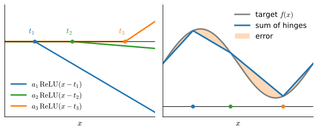
A one-dimensional construction illustrates the theorem. Consider a one-hidden-layer ReLU network on the real line. Each hidden unit contributes \(a_k \operatorname{ReLU}(w_k x + b_k)\) to the output: a hinge, flat on one side of the joint at \(x = -b_k/w_k\) and linear on the other. The network’s output is a sum of \(D\) such hinges, so it is a continuous piecewise linear function whose slope can change only at a joint: with \(D\) hidden units it has at most \(D\) joints and hence at most \(D+1\) linear pieces. Seen this way, approximating a continuous function reduces to approximating a curve with a polyline. Placing sufficiently many joints and choosing their slopes reduces the error to any prescribed tolerance (Figure 4.1.3). The exponential-width caveat below is visible here too: a very wiggly target needs a joint for every wiggle, one hidden unit apiece.

Figure 4.1.3: Universal approximation, one hinge at a time. Left: each of the three hidden units contributes a single hinge \(a_k \operatorname{ReLU}(x - t_k)\) whose joint \(t_k\) is marked on the horizontal axis. Right: adding the hinges to a base line yields a piecewise linear function with \(D+1 = 4\) pieces (blue) that tracks the smooth target (gray); the shaded band is the approximation error, which shrinks as more joints are added.

Width increases the number of pieces only linearly: one extra unit adds one joint. Depth is different. A second hidden layer applies its hinges not to \(x\) but to the piecewise linear output of the first layer, and composing with a hinge folds the graph: every existing piece that crosses the new joint is split in two. Each added layer can therefore roughly double the number of linear pieces, so \(k\) layers of width \(D\) can produce on the order of \((D+1)\,2^{k-1}\) pieces, a count that a single hidden layer could match only with exponentially many units. This multiplicative-versus-additive gap explains why depth can be more parameter-efficient than width. Both claims are easy to check numerically: below we evaluate randomly initialized ReLU MLPs on a dense one-dimensional grid, detect where the slope changes, and count the linear pieces.

def count_pieces(width, depth, rng, n=100001):
    x = onp.linspace(-4, 4, n).reshape(-1, 1)
    h = x
    for _ in range(depth):
        h = onp.maximum(h @ rng.standard_normal((h.shape[1], width))
                        + rng.standard_normal(width), 0)
    y = (h @ rng.standard_normal((width, 1))).squeeze()
    slope = onp.diff(y)
    tol = 1e-8 * onp.abs(slope).max() + 1e-12 * onp.abs(y).max()
    change = onp.abs(onp.diff(slope)) > tol
    new = change & ~onp.concatenate([[False], change[:-1]])
    return int(new.sum()) + 1
rng = onp.random.default_rng(0)
for depth in (1, 2, 3):
    mean = [round(sum(count_pieces(w, depth, rng) for _ in range(20)) / 20, 1)
            for w in (2, 4, 8, 16)]
    print(f'depth {depth}: mean pieces = {mean},  D+1 = {[3, 5, 9, 17]}')
depth 1: mean pieces = [2.8, 4.5, 7.8, 14.3],  D+1 = [3, 5, 9, 17]
depth 2: mean pieces = [3.2, 7.5, 14.2, 27.8],  D+1 = [3, 5, 9, 17]
depth 3: mean pieces = [3.0, 8.9, 19.5, 39.5],  D+1 = [3, 5, 9, 17]

The first row confirms the counting argument: with one hidden layer of width \(D\), the piece count never exceeds \(D+1\) (and typically comes close to it). The later rows show what happened for these seeded random networks: at each width, adding a layer increased the average piece count by a factor rather than by a fixed amount. This experiment does not establish a maximal count. Random weights fold less aggressively than hand-constructed networks used in depth separation results (Telgarsky 2016), and the expressivity claim rests on those constructions rather than on the sample averages above.

The third caveat—potentially impractical width—also motivates the distinction between depth and width (Goodfellow et al. 2016).

So the theorem tells us deep networks are expressive enough; it does not tell us they are the right tool, nor how to build them. For some problems other methods fit better (kernel methods, for instance, can solve regression problems exactly (Kimeldorf and Wahba 1971; Schölkopf et al. 2001)). Where a shallow network would need exponential width, a deep one can often represent the same function far more compactly, trading width for depth (Montúfar et al. 2014; Telgarsky 2016). This is one reason practitioners reach for depth rather than sheer width. The folding picture sketched above is the heart of these depth-separation results; exercise 6 asks you to turn it into an argument.

4.1.2 Activation Functions

Activation functions transform pre-activation signals into outputs and introduce nonlinearity into the network. Most are differentiable almost everywhere. We next examine several common choices.

4.1.2.1 ReLU Function

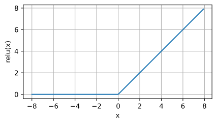
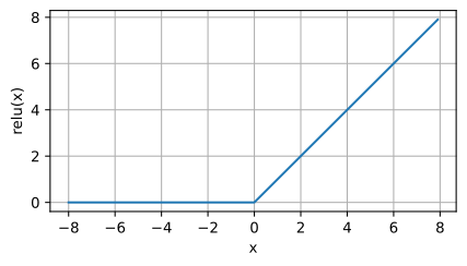
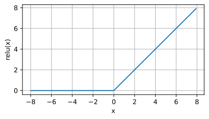
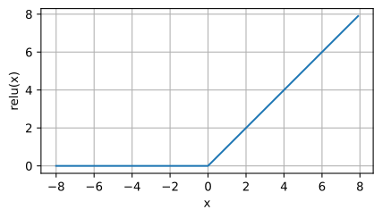
The most popular choice, due to both simplicity of implementation and its empirical performance across many predictive tasks, is the rectified linear unit (ReLU) (Nair and Hinton 2010). ReLU provides a very simple nonlinear transformation. Given an element \(x\), the function is defined as the maximum of that element and \(0\):

\[\operatorname{ReLU}(x) = \max(x, 0). \tag{4.1.2}\]

Informally, the ReLU function retains only positive elements and discards all negative elements by setting the corresponding activations to 0. To gain some intuition, we can plot the function. As you can see, the activation function is piecewise linear.

x = torch.arange(-8.0, 8.0, 0.1, requires_grad=True)
y = torch.relu(x)
d2l.plot(x.detach(), y.detach(), 'x', 'relu(x)', figsize=(5, 2.5))
x = tf.Variable(tf.range(-8.0, 8.0, 0.1), dtype=tf.float32)
y = tf.nn.relu(x)
d2l.plot(x.numpy(), y.numpy(), 'x', 'relu(x)', figsize=(5, 2.5))
x = jnp.arange(-8.0, 8.0, 0.1)
y = jax.nn.relu(x)
d2l.plot(x, y, 'x', 'relu(x)', figsize=(5, 2.5))
x = np.arange(-8.0, 8.0, 0.1)
x.attach_grad()
with autograd.record():
    y = npx.relu(x)
d2l.plot(x, y, 'x', 'relu(x)', figsize=(5, 2.5))
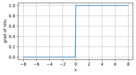
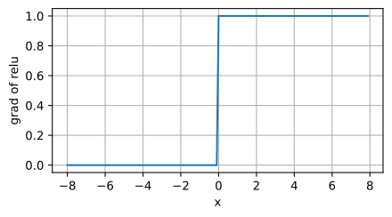
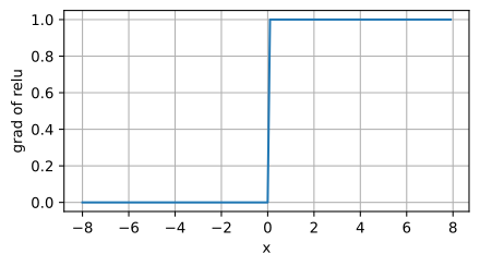
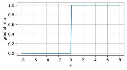
When the input is negative, the derivative of the ReLU function is 0, and when the input is positive, the derivative of the ReLU function is 1. Note that the ReLU function is not differentiable when the input takes value precisely equal to 0. The libraries used here return a derivative of 0 at the origin, one valid subgradient convention. For continuously distributed preactivations the choice affects a probability-zero event, but exact zeros do occur in computation, for example from zero-initialized biases or a preceding ReLU, and in such degenerate cases the convention can change whether a unit begins to move. We plot the derivative of the ReLU function below.

y.backward(torch.ones_like(x), retain_graph=True)
d2l.plot(x.detach(), x.grad, 'x', 'grad of relu', figsize=(5, 2.5))
with tf.GradientTape() as t:
    y = tf.nn.relu(x)
d2l.plot(x.numpy(), t.gradient(y, x).numpy(), 'x', 'grad of relu',
         figsize=(5, 2.5))
grad_relu = vmap(grad(jax.nn.relu))
d2l.plot(x, grad_relu(x), 'x', 'grad of relu', figsize=(5, 2.5))
y.backward()
d2l.plot(x, x.grad, 'x', 'grad of relu', figsize=(5, 2.5))
[21:25:40] /home/smola/mxnet/src/base.cc:48: GPU context requested, but no GPUs found.
The reason for using ReLU is that its derivatives are particularly well behaved: they are either zero or one. This makes optimization better behaved and it mitigated the well-documented problem of vanishing gradients that plagued previous versions of neural networks (more on this later).

This same flatness has a downside, however. Because the gradient is exactly zero for negative inputs, a unit whose pre-activation is pushed negative for every training example receives no gradient and stops updating: it becomes a permanently silent dead ReLU. To keep gradient flowing in that regime, several variants retain a nonzero slope for negative inputs. A common example is the parametrized ReLU (pReLU) (He et al. 2015), which adds a linear term so some information still gets through, even when the argument is negative:

\[\operatorname{pReLU}(x) = \max(0, x) + \alpha \min(0, x). \tag{4.1.3}\]

Here \(\alpha\) is a small slope (fixed for leaky ReLU, learned for pReLU).

4.1.2.2 Sigmoid Function

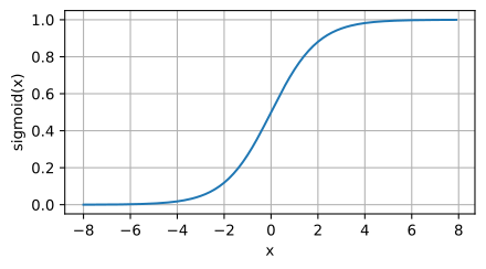
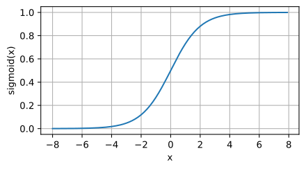
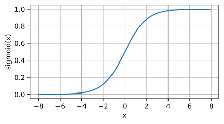
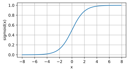
The sigmoid function transforms those inputs whose values lie in the domain \(\mathbb{R}\), to outputs that lie on the interval (0, 1). For that reason, the sigmoid is often called a squashing function: it squashes any input in the range (-inf, inf) to some value in the range (0, 1):

\[\operatorname{sigmoid}(x) = \frac{1}{1 + \exp(-x)}. \tag{4.1.4}\]

In the earliest neural networks, scientists were interested in modeling biological neurons that either fire or do not fire. Thus the pioneers of this field, going all the way back to McCulloch and Pitts, the inventors of the artificial neuron, focused on thresholding units (McCulloch and Pitts 1943). A thresholding activation takes value 0 when its input is below some threshold and value 1 when the input exceeds the threshold.

When attention shifted to gradient-based learning, the sigmoid function was a natural choice because it is a smooth, differentiable approximation to a thresholding unit. Sigmoids are still widely used as activation functions on the output units when we want to interpret the outputs as probabilities for binary classification problems: you can think of the sigmoid as a special case of the softmax, namely the softmax over the two logits \(\{x, 0\}\). However, the sigmoid has largely been replaced by the simpler and more easily trainable ReLU for most use in hidden layers. Much of this has to do with the fact that the sigmoid poses challenges for optimization (LeCun et al. 1998) since its gradient vanishes for large positive and negative arguments. This can lead to plateaus that are difficult to escape from. Nonetheless sigmoids are important. In later chapters (e.g., Section 12.1) on recurrent neural networks, we will describe architectures that use sigmoid units to control the flow of information across time.

Below, we plot the sigmoid function. Note that when the input is close to 0, the sigmoid function approaches a linear transformation.

y = torch.sigmoid(x)
d2l.plot(x.detach(), y.detach(), 'x', 'sigmoid(x)', figsize=(5, 2.5))
y = tf.nn.sigmoid(x)
d2l.plot(x.numpy(), y.numpy(), 'x', 'sigmoid(x)', figsize=(5, 2.5))
y = jax.nn.sigmoid(x)
d2l.plot(x, y, 'x', 'sigmoid(x)', figsize=(5, 2.5))
with autograd.record():
    y = npx.sigmoid(x)
d2l.plot(x, y, 'x', 'sigmoid(x)', figsize=(5, 2.5))
The derivative of the sigmoid function is given by the following equation:

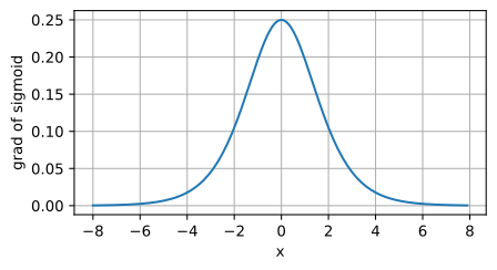
\[\frac{d}{dx} \operatorname{sigmoid}(x) = \frac{\exp(-x)}{(1 + \exp(-x))^2} = \operatorname{sigmoid}(x)\left(1-\operatorname{sigmoid}(x)\right). \tag{4.1.5}\]

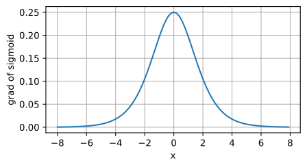
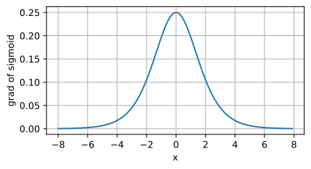
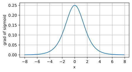
The derivative of the sigmoid function is plotted below. Note that when the input is 0, the derivative of the sigmoid function reaches a maximum of 0.25. As the input diverges from 0 in either direction, the derivative approaches 0.

# Clear out previous gradients
x.grad.zero_()
y.backward(torch.ones_like(x),retain_graph=True)
d2l.plot(x.detach(), x.grad, 'x', 'grad of sigmoid', figsize=(5, 2.5))
with tf.GradientTape() as t:
    y = tf.nn.sigmoid(x)
d2l.plot(x.numpy(), t.gradient(y, x).numpy(), 'x', 'grad of sigmoid',
         figsize=(5, 2.5))
grad_sigmoid = vmap(grad(jax.nn.sigmoid))
d2l.plot(x, grad_sigmoid(x), 'x', 'grad of sigmoid', figsize=(5, 2.5))
y.backward()
d2l.plot(x, x.grad, 'x', 'grad of sigmoid', figsize=(5, 2.5))
4.1.2.3 Tanh Function

Like the sigmoid function, the tanh (hyperbolic tangent) function also squashes its inputs, transforming them into elements on the interval between \(-1\) and \(1\):

\[\operatorname{tanh}(x) = \frac{1 - \exp(-2x)}{1 + \exp(-2x)}. \tag{4.1.6}\]

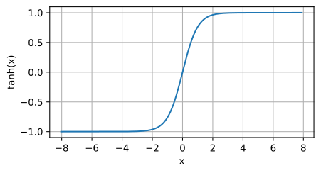
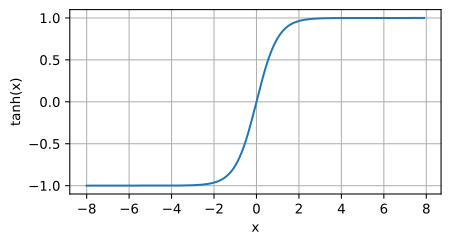
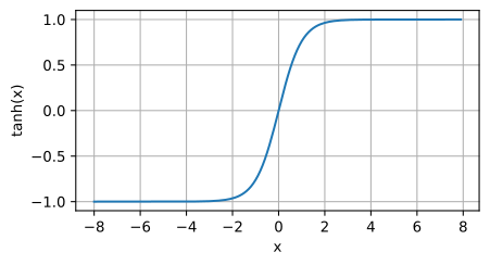
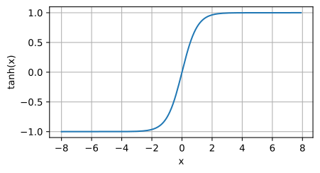
We plot the tanh function below. Note that as input nears 0, the tanh function approaches a linear transformation. Although the shape of the function is similar to that of the sigmoid function, the tanh function exhibits point symmetry about the origin of the coordinate system.

y = torch.tanh(x)
d2l.plot(x.detach(), y.detach(), 'x', 'tanh(x)', figsize=(5, 2.5))
y = tf.nn.tanh(x)
d2l.plot(x.numpy(), y.numpy(), 'x', 'tanh(x)', figsize=(5, 2.5))
y = jax.nn.tanh(x)
d2l.plot(x, y, 'x', 'tanh(x)', figsize=(5, 2.5))
with autograd.record():
    y = np.tanh(x)
d2l.plot(x, y, 'x', 'tanh(x)', figsize=(5, 2.5))
The derivative of the tanh function is:

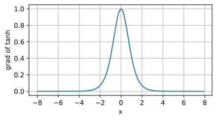
\[\frac{d}{dx} \operatorname{tanh}(x) = 1 - \operatorname{tanh}^2(x). \tag{4.1.7}\]

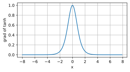
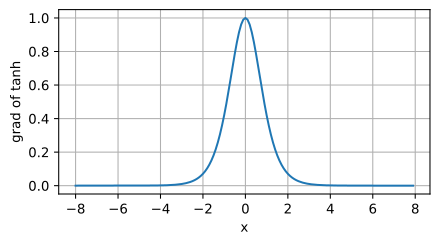
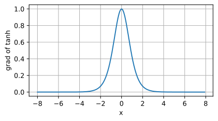
It is plotted below. As the input nears 0, the derivative of the tanh function approaches a maximum of 1. And as we saw with the sigmoid function, as input moves away from 0 in either direction, the derivative of the tanh function approaches 0.

# Clear out previous gradients
x.grad.zero_()
y.backward(torch.ones_like(x),retain_graph=True)
d2l.plot(x.detach(), x.grad, 'x', 'grad of tanh', figsize=(5, 2.5))
with tf.GradientTape() as t:
    y = tf.nn.tanh(x)
d2l.plot(x.numpy(), t.gradient(y, x).numpy(), 'x', 'grad of tanh',
         figsize=(5, 2.5))
grad_tanh = vmap(grad(jax.nn.tanh))
d2l.plot(x, grad_tanh(x), 'x', 'grad of tanh', figsize=(5, 2.5))
y.backward()
d2l.plot(x, x.grad, 'x', 'grad of tanh', figsize=(5, 2.5))
4.1.3 Summary and Discussion

Nonlinear activations prevent stacked affine layers from reducing to one affine map. They make MLPs expressive enough for nonlinear decision boundaries, while the universal approximation theorem supplies only a representational guarantee, not an optimization or generalization guarantee.

A key reason ReLU displaced sigmoid and tanh in hidden layers is that it is so much more amenable to optimization. One could argue that this was one of the innovations that helped the resurgence of deep learning in the early 2010s. Research on activation functions has not stopped, though, and you will meet newer ones once we reach the Transformer architectures later in the book. The most common are GELU (Gaussian error linear unit), \(x \Phi(x)\), where \(\Phi\) is the standard Gaussian cumulative distribution function (Hendrycks and Gimpel 2016), used in BERT and GPT-2-style models; Swish, \(x \operatorname{sigmoid}(\beta x)\) (Ramachandran et al. 2017); and SwiGLU (Shazeer 2020), a gated variant that is the default feedforward nonlinearity in recent large language models such as PaLM, LLaMA, and Mistral. For now, ReLU remains the sensible default for the models we build next.

4.1.4 Exercises

  1. Show that adding layers to a linear deep network, i.e., a network without nonlinearity \(\sigma\) can never increase the expressive power of the network. Give an example where it actively reduces it.
  2. Find weights for a two-hidden-unit ReLU network that computes XOR, and verify them on the four inputs. (You may reuse the construction in Figure 4.1.2, but try to derive your own first.) Can a single ReLU unit compute XOR? Why or why not?
  3. Compute the derivative of the pReLU activation function.
  4. Compute the derivative of the Swish activation function \(x \operatorname{sigmoid}(\beta x)\).
  5. Show that an MLP using only ReLU (or pReLU) constructs a continuous piecewise linear function.
  6. Explain intuitively why composing ReLU layers can roughly double the number of linear pieces the network represents with each added layer, so that depth can yield exponentially many pieces, whereas width yields only linearly many. (This is the depth-versus-width gap behind the universal-approximation caveat above.)
  7. Sigmoid and tanh are very similar.
    1. Show that \(\operatorname{tanh}(x) + 1 = 2 \operatorname{sigmoid}(2x)\).
    2. Prove that the function classes parametrized by both nonlinearities are identical. Hint: affine layers have bias terms, too.
  8. Assume that we have a nonlinearity that applies to one minibatch at a time, such as the batch normalization (Ioffe and Szegedy 2015) (covered in Section 7.3). What kinds of problems do you expect this to cause?
  9. Provide an example where the gradients vanish for the sigmoid activation function.