%matplotlib inline
from d2l import torch as d2l
import numpy as np
from scipy import integrate, optimize28.2 Divergences and Distances Between Distributions
Many learning problems compare two probability distributions. A language model compares next-token distributions with corpus data; a VAE compares an approximate posterior with a target posterior; GANs compare generated and real samples; and diffusion models compare score fields. The chosen notion of discrepancy determines the training objective, its gradients, and its typical failure modes.
In Section 28.1 we built one such notion, the Kullback–Leibler divergence, and saw that minimizing it is maximum likelihood. This section develops three broader families: f-divergences, which average a convex function of the density ratio \(p/q\) (KL, reverse KL, \(\chi^2\), Hellinger, Jensen–Shannon); integral probability metrics, which measure the largest gap in expectation any test function from a chosen class can detect (total variation, MMD, Wasserstein-1); and optimal transport distances, which measure how far probability mass must move. We derive the structural results that organize the families: Jensen for non-negativity, Fenchel duality for the adversarial (f-GAN) view, Pinsker’s inequality tying total variation to KL, and Kantorovich–Rubinstein duality with the one-dimensional closed form for Wasserstein. We close with the score: the gradient \(\nabla_{\mathbf{x}} \log p(\mathbf{x})\) of the log-density with respect to the data, which is central to Section 29.4. A final table relates common generative objectives to their associated divergences.
As in Section 28.1, every logarithmic quantity is in nats (natural logarithms); bits are a fixed \(\ln 2\) rescaling. Not every divergence carries units, though: KL, reverse KL, and Jensen–Shannon are in nats, but total variation, \(\chi^2\), and squared Hellinger contain no logarithm and are dimensionless, and transport distances carry the units of the sample space itself. The numerical examples use NumPy and SciPy.
%matplotlib inline
from d2l import tensorflow as d2l
import numpy as np
from scipy import integrate, optimize%matplotlib inline
from d2l import jax as d2l
import numpy as np
from scipy import integrate, optimize%matplotlib inline
from d2l import mxnet as d2l
import numpy as np
from scipy import integrate, optimize28.2.1 Divergences and the f-Divergence Family
28.2.1.1 Axioms, Metrics, and Three Families
A divergence provides a minimal notion of separation between distributions. It is a function \(D(P, Q) \geq 0\) with
\[ D(P, Q) = 0 \quad \textrm{if and only if} \quad P = Q, \]
and nothing more. Compare this with the norms of Section 1.3: a metric additionally demands symmetry, \(D(P, Q) = D(Q, P)\), and the triangle inequality, \(D(P, R) \leq D(P, Q) + D(Q, R)\). We drop both on purpose, because the most useful divergence in machine learning fails both. The KL divergence of Section 28.1 is asymmetric: for \(P = \mathcal{N}(0, 1)\) and \(Q = \mathcal{N}(0, 4)\) the closed form Equation 28.1.5 gives \(D_{\textrm{KL}}(P\|Q) \approx 0.318\) nats but \(D_{\textrm{KL}}(Q\|P) \approx 0.807\) nats. And KL fails the triangle inequality too, not because it is asymmetric (asymmetric functions can perfectly well satisfy a directed triangle inequality; such quasimetrics include one-way travel times), but because it scales like a squared distance: for unit Gaussians centered at \(0\), \(1\), and \(2\), the same closed form gives \(D_{\textrm{KL}} = \tfrac{1}{2}\) for each adjacent pair but \(2\) for the outer pair, and \(2 > \tfrac{1}{2} + \tfrac{1}{2}\) in either argument order. The asymmetry is informative: Section 28.2.2.2 shows that the direction of KL is a modeling decision that changes what the fitted model does. Still, some divergences are genuine metrics (total variation, the Hellinger distance, and the Wasserstein distances among them), and when a problem needs the triangle inequality (coupling arguments, convergence proofs), those are the ones to reach for.
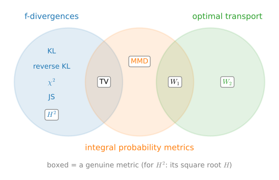
The divergences that matter in deep learning organize into three families, sketched in Figure 28.2.1:
- f-divergences average a convex function of the density ratio \(p(x)/q(x)\). They are the information-theoretic family: KL, reverse KL, \(\chi^2\), squared Hellinger, total variation, Jensen–Shannon.
- Integral probability metrics (IPMs) report the largest gap in expectation \(E_P[f] - E_Q[f]\) over a class of test functions \(f\). They are the statistician’s family, computable from samples alone, and include total variation, maximum mean discrepancy (MMD), and Wasserstein-1.
- Optimal transport distances measure the minimum cost of physically moving the mass of \(P\) onto \(Q\). They use the geometry of the sample space and often vary when bounded f-divergences saturate on disjoint supports; a geometry-sensitive characteristic-kernel MMD can also vary there.
The families intersect: total variation is both an f-divergence and an IPM, and Wasserstein-1 is both an IPM and a transport distance. The intersections are where the most useful theorems live.
28.2.1.2 The f-Divergence Template
Many common divergences share one definition. Let \(f : (0, \infty) \to \mathbb{R}\) be convex with \(f(1) = 0\), and let \(P\) and \(Q\) have densities (or p.m.f.s) \(p\) and \(q\) with \(p(x) = 0\) wherever \(q(x) = 0\). The f-divergence with generator \(f\) is (Csiszár 1967)
\[ D_f(P\|Q) = E_{x \sim Q}\!\left[ f\!\left( \frac{p(x)}{q(x)} \right) \right]. \tag{28.2.1}\]
This formula assumes \(P\) is absolutely continuous with respect to \(Q\), written \(P\ll Q\). For general measures, decompose \(P\) into a part with density \(p/q\) relative to \(Q\) and a singular part \(P_\perp\). The extended definition adds \(f'(\infty)P_\perp(\mathcal X)\), where \(f'(\infty)=\lim_{t\to\infty}f(t)/t\). Thus support mismatch may give a finite boundary contribution for some generators and \(+\infty\) for forward KL.
For discrete distributions, the same boundary terms follow from the standard conventions \(0 \cdot f(0/0) = 0\) and, for outcomes with \(q(x) = 0 < p(x)\), a contribution \(p(x)\, f'(\infty)\) with \(f'(\infty) = \lim_{t \to \infty} f(t)/t\), possibly infinite; the disjoint-support evaluations of Section 28.2.3.3 use this extension.
The density ratio \(u = p/q\) says, point by point, how \(P\) over- or under-represents \(x\) relative to \(Q\); the generator \(f\) decides how to score that discrepancy (\(f(1) = 0\): no discrepancy, no score); and the expectation under \(Q\) aggregates. Convexity of \(f\) is exactly what makes the score sound:
Proposition (non-negativity). For any convex \(f\) with \(f(1) = 0\),
\[ D_f(P\|Q) \geq 0, \]
and if \(f\) is strictly convex at \(1\), then \(D_f(P\|Q) = 0\) if and only if \(P = Q\).
Proof. Jensen’s inequality (Section 26.3.3) applied to the convex \(f\) and the random variable \(u(x) = p(x)/q(x)\) under \(x \sim Q\):
\[ D_f(P\|Q) = E_Q[f(u)] \geq f(E_Q[u]) = f\!\left( \sum_x q(x) \frac{p(x)}{q(x)} \right) = f(1) = 0. \]
If \(f\) is strictly convex at \(1\), equality forces \(u\) to be constant \(Q\)-almost surely; a constant density ratio between two normalized distributions must equal \(1\), i.e., \(P = Q\). \(\blacksquare\)
The proof is Gibbs’ inequality from Section 28.1, run for every generator at once: taking \(f(u) = u \log u\) recovers \(E_Q[(p/q)\log(p/q)] = E_P[\log(p/q)] = D_{\textrm{KL}}(P\|Q)\) and the proof specializes to the one we gave there.
28.2.1.3 Common f-Divergence Generators
Each row of the following table is one choice of \(f\); the curves are plotted in Figure 28.2.2.
| Divergence | Generator \(f(u)\) | Symmetric? | Metric? |
|---|---|---|---|
| Kullback–Leibler (forward) | \(u \log u\) | no | no |
| reverse KL | \(-\log u\) | no | no |
| Pearson \(\chi^2\) | \((u - 1)^2\) | no | no |
| squared Hellinger \(H^2\) | \((\sqrt{u} - 1)^2\) | yes | \(H\) is a metric |
| total variation | \(\tfrac{1}{2}\lvert u - 1 \rvert\) | yes | yes |
| Jensen–Shannon | \(\tfrac{u}{2} \log u - \tfrac{u+1}{2} \log \tfrac{u+1}{2}\) | yes | \(\sqrt{\textrm{JS}}\) is a metric |
| \(\alpha\)-divergence (\(\alpha \neq 0, 1\)) | \(\dfrac{u^\alpha-\alpha u+\alpha-1}{\alpha(\alpha-1)}\) | no | no |
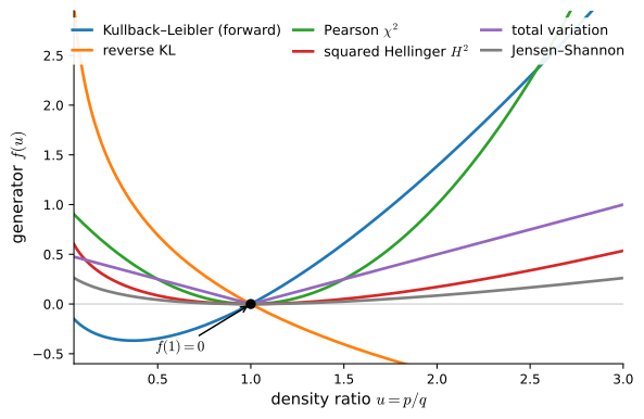
Reverse KL is KL with its arguments swapped: \(D_f(P\|Q)\) with \(f(u) = -\log u\) equals \(E_Q[\log(q/p)] = D_{\textrm{KL}}(Q\|P)\), so the asymmetry of KL becomes a choice of generator rather than a quirk (Exercise 1). Total variation with \(f(u) = \tfrac{1}{2}|u - 1|\) unwinds to \(\tfrac{1}{2}\sum_x |p(x) - q(x)|\), half the \(\ell_1\) distance between the probability vectors; we study it in Section 28.2.3.1. And the Jensen–Shannon divergence (Lin 1991) is the natural symmetrization of KL. Writing \(M = \tfrac{1}{2}(P + Q)\) for the even mixture,
\[ \textrm{JS}(P, Q) = \frac{1}{2} D_{\textrm{KL}}(P \,\|\, M) + \frac{1}{2} D_{\textrm{KL}}(Q \,\|\, M). \tag{28.2.2}\]
Each distribution is compared with the mixture \(M\), which dominates both; comparing them with each other directly would risk the infinities of KL when supports differ. As a result JS is symmetric, always finite, and bounded: \(0 \leq \textrm{JS}(P, Q) \leq \log 2\), with the upper bound attained exactly when \(P\) and \(Q\) have disjoint supports (each \(\log(p/m)\) becomes \(\log 2\) on its own support); its square root is moreover a genuine metric (Endres and Schindelin 2003), as the gallery table records. That boundedness becomes a limitation in Section 28.2.3.3: on disjoint supports JS is constant at \(\log 2\), so it provides no gradient. Expanding Equation 28.2.2 in terms of the ratio \(u = p/q\) produces the generator in the table (Exercise 1 checks a similar unwinding).
The table’s last row is a family within the family (Amari 2016). For each \(\alpha \neq 0, 1\) use the normalized generator
\[ f_\alpha(u)=\frac{u^\alpha-\alpha u+\alpha-1}{\alpha(\alpha-1)}. \]
It is convex with \(f_\alpha(1)=0\), and its pointwise limits are \(u\log u-u+1\) as \(\alpha\to1\) and \(-\log u+u-1\) as \(\alpha\to0\). The added linear terms integrate to zero because \(E_Q[p/q-1]=0\), so the resulting divergences are forward and reverse KL. At \(\alpha=\tfrac12\) it gives twice the squared Hellinger divergence under the table’s convention. The shorter generator \((u^\alpha-1)/(\alpha(\alpha-1))\) defines the same divergence for fixed \(\alpha\)—the two differ only by a multiple of \(u-1\)—but it does not have the claimed pointwise limits. Closely related is the Rényi divergence (Rényi 1961), the form that appears in applications,
\[ D_\alpha(P\|Q) = \frac{1}{\alpha - 1} \log \sum_x p(x)^\alpha\, q(x)^{1-\alpha}. \tag{28.2.3}\]
The outer logarithm breaks the template, so Rényi is not an f-divergence. But it is a monotone increasing function of one: the sum inside is \(E_Q[(p/q)^\alpha] = 1 + \alpha(\alpha - 1)\, D_{f_\alpha}(P\|Q)\), and \(t \mapsto \frac{1}{\alpha-1}\log\big(1 + \alpha(\alpha-1)\,t\big)\) is increasing for \(\alpha > 0\), so non-negativity and the data-processing inequality (Section 28.2.3.1) transfer verbatim. One application: Rényi differential privacy (Mironov 2017) measures a randomized algorithm’s privacy loss in \(D_\alpha\), which adds exactly across independent compositions. For the full atlas of the family (limits, orderings, and the fact that \(D_\alpha\) is nondecreasing in \(\alpha\)) see Erven and Harremoës (2014).
We evaluate each divergence on the same pair of categorical distributions used in Section 28.1, \(P = (0.6, 0.3, 0.1)\) and \(Q = (0.2, 0.5, 0.3)\), in both argument orders.
def f_divergence(f, p, q):
    """D_f(P||Q) = sum_x q(x) f(p(x)/q(x)); nats for KL/JS, else unitless."""
    return np.sum(q * f(p / q))

generators = {
    'KL':          lambda u: u * np.log(u),
    'reverse KL':  lambda u: -np.log(u),
    'chi^2':       lambda u: (u - 1) ** 2,
    'Hellinger^2': lambda u: (np.sqrt(u) - 1) ** 2,
    'TV':          lambda u: 0.5 * np.abs(u - 1),
    'JS':          lambda u: u / 2 * np.log(u) - (u + 1) / 2 * np.log((u + 1) / 2),
}

p = np.array([0.6, 0.3, 0.1])
q = np.array([0.2, 0.5, 0.3])
for name, f in generators.items():
    print(f'{name:12s} D_f(P||Q) = {f_divergence(f, p, q):.4f}   '
          f'D_f(Q||P) = {f_divergence(f, q, p):.4f}')

m = (p + q) / 2
js_mix = 0.5 * f_divergence(generators['KL'], p, m) \
    + 0.5 * f_divergence(generators['KL'], q, m)
print(f'JS via the mixture formula: {js_mix:.4f}')
KL D_f(P||Q) = 0.3961 D_f(Q||P) = 0.3653
reverse KL D_f(P||Q) = 0.3653 D_f(Q||P) = 0.3961
chi^2 D_f(P||Q) = 1.0133 D_f(Q||P) = 0.8000
Hellinger^2 D_f(P||Q) = 0.1862 D_f(Q||P) = 0.1862
TV D_f(P||Q) = 0.4000 D_f(Q||P) = 0.4000
JS D_f(P||Q) = 0.0911 D_f(Q||P) = 0.0911
JS via the mixture formula: 0.0911The KL row is asymmetric (\(0.3961\) vs. \(0.3653\) nats, the same two numbers as in Section 28.1), and the reverse-KL row is the KL row with its columns swapped, exactly as the generator algebra predicts. The \(\chi^2\) row is also asymmetric (\(1.0133\) vs. \(0.8000\)). Hellinger, TV, and JS are symmetric, JS comfortably under its \(\log 2 \approx 0.693\) ceiling at \(0.0911\) nats, and the mixture formula Equation 28.2.2 reproduces the generator’s value exactly.
One more structural fact ties the family together. Adding \(c\,(u - 1)\) to any generator changes nothing, since \(E_Q[c\,(p/q - 1)] = c\,(1 - 1) = 0\) (Exercise 1), so each \(f\) is really an equivalence class, and what distinguishes divergences locally is the curvature \(f''(1)\). For \(f\) twice continuously differentiable near \(1\) and density ratios uniformly near \(1\), a second-order expansion of Equation 28.2.1 around \(u = 1\) makes every such f-divergence the same quadratic to leading order,
\[ D_f(P\|Q) \approx \frac{f''(1)}{2}\, \chi^2(P\|Q), \]
with error third order in the deviation of \(p/q\) from \(1\) (Erven and Harremoës 2014): \(f''(1) = 1\) for KL and reverse KL, \(2\) for \(\chi^2\), \(\tfrac{1}{2}\) for \(H^2\), \(\tfrac{1}{4}\) for JS. Near equality all smooth f-divergences agree. This shared local quadratic is the Fisher-information geometry behind natural-gradient methods (Amari 1998): for a parametric family \(q_{\boldsymbol{\theta}}\), the quadratic’s Hessian in \(\boldsymbol{\theta}\) is \(f''(1)\) times the Fisher information matrix that Section 27.3 develops as the curvature of the log-likelihood. The families disagree only about distant distributions, which is precisely the regime early in training.
28.2.2 Duality: The Variational View
The definition Equation 28.2.1 has a practical flaw: it needs the densities. A generative model can sample, and the data are samples, but neither source provides \(p(x)/q(x)\). Convex duality gives a variational equality when the critic ranges over a sufficiently rich measurable class and the required expectations are finite. Restricting the critic to a neural family turns that equality into a lower bound; finite-sample estimation and incomplete optimization introduce further gaps.
28.2.2.1 The Fenchel Conjugate and the f-GAN Bound
Recall the convex conjugate from Section 26.3.5.3: for a convex \(f\),
\[ f^*(t) = \sup_{u > 0}\, \big( ut - f(u) \big), \]
and for closed convex \(f\) the biconjugation theorem gives back \(f(u) = \sup_t \big( ut - f^*(t) \big)\). Geometrically, \(-f^*(t)\) is the intercept of the tangent line to \(f\) with slope \(t\), and biconjugation says a convex function is the upper envelope of its tangent lines (Figure 28.2.3). Keeping one tangent instead of the envelope gives the Fenchel–Young inequality
\[ f(u) \geq ut - f^*(t) \quad \textrm{for all } t, \tag{28.2.4}\]
with equality when \(t\) is the slope of \(f\) at \(u\), i.e., \(t = f'(u)\).
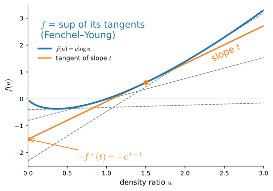
Now do this pointwise inside the divergence, letting the slope vary with \(x\): choose any function \(T(x)\) (the critic) and apply Equation 28.2.4 at \(u = p(x)/q(x)\), \(t = T(x)\).
Proposition (f-GAN variational bound). For every function \(T\),
\[ D_f(P\|Q) \;\geq\; E_{x \sim P}[T(x)] - E_{x \sim Q}[f^*(T(x))], \tag{28.2.5}\]
and the bound is attained at the optimal critic \(T^\star(x) = f'(p(x)/q(x))\), so the supremum over \(T\) equals \(D_f(P\|Q)\) (Nowozin et al. 2016).
Proof. Multiply Equation 28.2.4 at \(u = p(x)/q(x)\), \(t = T(x)\) by \(q(x) \geq 0\):
\[ q(x)\, f\!\left(\frac{p(x)}{q(x)}\right) \;\geq\; p(x)\, T(x) - q(x)\, f^*(T(x)). \]
Summing (or integrating) over \(x\) gives Equation 28.2.5. Since Fenchel–Young holds with equality at \(t = f'(u)\), the choice \(T^\star(x) = f'(p(x)/q(x))\) makes the inequality an equality pointwise, hence in expectation. \(\blacksquare\)
Look at what the right-hand side of Equation 28.2.5 asks for: an average of \(T\) over samples from \(P\) and an average of \(f^*(T)\) over samples from \(Q\); neither average requires densities. Parameterizing \(T\) by a neural network makes the bound estimable and optimizable from minibatches. In the f-GAN objective, the critic maximizes the bound, which equals the true divergence at optimality, while the generator controlling \(Q\) minimizes it. The original GAN of Goodfellow et al. (2014) is the special case corresponding to the Jensen–Shannon generator: at the optimal discriminator, the classic GAN value function equals \(2\,\textrm{JS}(P, Q) - \log 4\). For the KL generator \(f(u) = u \log u\) the conjugate is \(f^*(t) = e^{t-1}\), giving \(D_{\textrm{KL}}(P\|Q) \geq E_P[T] - E_Q[e^{T-1}]\), a bound we will meet again, tightened into Donsker–Varadhan form, when Section 28.3 estimates mutual information variationally.
Two practical caveats remain. The bound is tight only at the optimal critic, so with an undertrained critic the game systematically underestimates the divergence: adversarial losses are biased low. And the critic that attains the bound depends on the density ratio, so on disjoint supports (where the ratio is \(0\) or \(\infty\)) optimal critics saturate, previewing the gradient problems discussed in Section 28.2.3.3.
We can verify the proposition exactly on a finite categorical example, where expectations reduce to sums. Use the pair from before, with the \(\chi^2\) generator \(f(u) = (u-1)^2\). Its conjugate is \(f^*(t) = t + t^2/4\) and the optimal critic is \(T^\star = 2(p/q - 1)\) (Exercise 2 derives both). One fine point: \(t + t^2/4\) is the conjugate taken over all \(u \in \mathbb{R}\); over the generator’s true domain \(u \in (0, \infty)\) the supremum flattens to \(f^*(t) = -1\) for \(t \leq -2\). Using the larger \(\mathbb{R}\)-conjugate is safe (a bigger \(f^*\) only lowers the bound Equation 28.2.5) and costs nothing at the optimum, where \(T^\star = 2(p/q - 1) > -2\) automatically. On three outcomes a critic is a vector of three numbers.
chi_sq = generators['chi^2']            # f(u) = (u - 1)^2
f_star = lambda t: t + t ** 2 / 4       # its convex conjugate

def fgan_bound(T, p, q):
    """E_P[T] - E_Q[f*(T)]: a lower bound on D_f for any critic T."""
    return np.sum(p * T) - np.sum(q * f_star(T))

T_star = 2 * (p / q - 1)                # the optimal critic f'(p/q)
print(f'exact chi^2(P||Q)           = {f_divergence(chi_sq, p, q):.4f}')
print(f'bound at the optimal critic = {fgan_bound(T_star, p, q):.4f}')
rng = np.random.default_rng(42)
for scale in (0.5, 1.0, 2.0):
    T = T_star + scale * rng.standard_normal(3)
    print(f'bound at a perturbed critic (scale {scale}): '
          f'{fgan_bound(T, p, q):.4f}')
exact chi^2(P||Q) = 1.0133
bound at the optimal critic = 1.0133
bound at a perturbed critic (scale 0.5): 0.9678
bound at a perturbed critic (scale 1.0): 0.3661
bound at a perturbed critic (scale 2.0): 0.9600The optimal critic reproduces the exact divergence, \(1.0133\), to every printed digit, and every random perturbation of it (\(0.9678\), \(0.3661\), \(0.9600\)) gives a strictly smaller value. The variational objective equals the true divergence only at the optimal critic.
28.2.2.2 Forward vs. Reverse KL: Mode-Covering vs. Mode-Seeking
When fitting a model \(Q_\theta\) to a target \(P\), the two directions of KL ask for different things:
- Forward KL, \(D_{\textrm{KL}}(P \,\|\, Q_\theta) = E_P[\log(p/q_\theta)]\), samples from the truth. Wherever \(P\) puts mass, \(q_\theta\) appears in a denominator: if \(q_\theta(x) \to 0\) while \(p(x) > 0\), the divergence blows up. Forward KL is zero-avoiding: the model must cover every mode of the data, even at the price of smearing mass over regions \(P\) never visits.
- Reverse KL, \(D_{\textrm{KL}}(Q_\theta \,\|\, P) = E_{Q_\theta}[\log(q_\theta/p)]\), samples from the model. Now \(p\) is the denominator: the model is punished for putting mass where the truth has none, while modes it never visits leave the objective untouched. Reverse KL is zero-forcing: the model concentrates on the mass it can explain and assigns little probability to the rest.
The two directions correspond to the two great fitting paradigms. Maximum likelihood is forward KL minimization: we proved in Section 27.3.2.1 that the average negative log-likelihood is the cross-entropy from the empirical distribution to the model. Variational inference and the ELBO (Section 27.3.5) minimize the reverse KL from the approximate posterior to the true one, which is why variational posteriors are characteristically too narrow and why VAEs can drop modes.
When the model family contains the target, both directions agree on the answer. The two directions differ for a misspecified family; the simplest instance is fitting a single Gaussian to a bimodal target. For the forward direction the optimum is fully characterized:
Proposition (forward KL fits moments). Over the Gaussian family \(Q = \mathcal{N}(\mu, \sigma^2)\), the forward divergence \(D_{\textrm{KL}}(P \,\|\, Q)\) is minimized at
\[ \mu^* = E_P[X], \qquad (\sigma^*)^2 = \mathrm{Var}_P(X). \]
Proof. For \(P\) with a density and finite differential entropy \(h(P)\), \(D_{\textrm{KL}}(P\|Q) = -h(P) - E_P[\log q(X)]\) with \(h(P)\) fixed, so we maximize \(E_P[\log q(X)] = -\tfrac{1}{2}\log(2\pi\sigma^2) - E_P[(X-\mu)^2]/(2\sigma^2)\). For any \(\sigma\), \(E_P[(X-\mu)^2] = \mathrm{Var}_P(X) + (E_P[X] - \mu)^2\) is minimized at \(\mu = E_P[X]\); substituting \(v = \mathrm{Var}_P(X)\) and setting the \(\sigma^2\)-derivative of \(-\tfrac{1}{2}\log\sigma^2 - v/(2\sigma^2)\) to zero gives \(\sigma^2 = v\). \(\blacksquare\)
(The same argument runs for any exponential family: the forward-KL projection matches expected sufficient statistics, the M-projection of information geometry (Amari 2016).) The reverse direction has no such closed form and can have local optima associated with different modes. The following example computes both fits for the mixture \(P = 0.7\,\mathcal{N}(-2, 0.6^2) + 0.3\,\mathcal{N}(2, 0.6^2)\), evaluating each KL by quadrature on a grid and minimizing over \((\mu, \log\sigma)\) with a derivative-free optimizer.
w, mus, sigmas = np.array([0.7, 0.3]), np.array([-2.0, 2.0]), np.array([0.6, 0.6])
x = np.linspace(-8.0, 8.0, 4001)

def log_p(x):
    comps = np.stack([np.log(wi) - 0.5 * np.log(2 * np.pi * si ** 2)
                      - (x - mi) ** 2 / (2 * si ** 2)
                      for wi, mi, si in zip(w, mus, sigmas)])
    cmax = comps.max(axis=0)
    return cmax + np.log(np.exp(comps - cmax).sum(axis=0))

def log_q(x, theta):
    mu, log_sigma = theta
    return (-0.5 * np.log(2 * np.pi) - log_sigma
            - (x - mu) ** 2 / (2 * np.exp(2 * log_sigma)))

def kl(log_a, log_b):
    """D_KL(A||B) on the grid, by quadrature; in nats."""
    return integrate.trapezoid(np.exp(log_a) * (log_a - log_b), x)

fwd = lambda th: kl(log_p(x), log_q(x, th))     # D_KL(P || Q_theta)
rev = lambda th: kl(log_q(x, th), log_p(x))     # D_KL(Q_theta || P)

th_fwd = optimize.minimize(fwd, x0=[0.0, 0.0], method='Nelder-Mead').x
th_rev = optimize.minimize(rev, x0=[0.0, 0.0], method='Nelder-Mead').x
th_rev2 = optimize.minimize(rev, x0=[2.5, -0.5], method='Nelder-Mead').x

for name, th, val in [('forward KL', th_fwd, fwd(th_fwd)),
                      ('reverse KL', th_rev, rev(th_rev)),
                      ('reverse KL, 2nd start', th_rev2, rev(th_rev2))]:
    print(f'{name:22s} mu = {th[0]:+.3f}, sigma = {np.exp(th[1]):.3f}, '
          f'KL = {val:.3f} nats')

d2l.plot(x, [np.exp(log_p(x)), np.exp(log_q(x, th_fwd)),
             np.exp(log_q(x, th_rev))], 'x', 'density',
         legend=['target P (mixture)', 'forward-KL fit', 'reverse-KL fit'],
figsize=(6, 3))forward KL mu = -0.800, sigma = 1.929, KL = 0.558 nats
reverse KL mu = -1.998, sigma = 0.603, KL = 0.356 nats
reverse KL, 2nd start mu = +1.995, sigma = 0.607, KL = 1.202 nats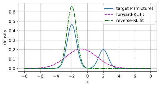
forward KL             mu = -0.800, sigma = 1.929, KL = 0.558 nats
reverse KL             mu = -1.998, sigma = 0.603, KL = 0.356 nats
reverse KL, 2nd start  mu = +1.995, sigma = 0.607, KL = 1.202 nats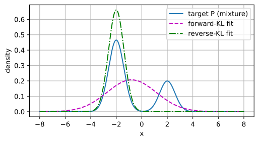
forward KL             mu = -0.800, sigma = 1.929, KL = 0.558 nats
reverse KL             mu = -1.998, sigma = 0.603, KL = 0.356 nats
reverse KL, 2nd start  mu = +1.995, sigma = 0.607, KL = 1.202 nats
forward KL             mu = -0.800, sigma = 1.929, KL = 0.558 nats
reverse KL             mu = -1.998, sigma = 0.603, KL = 0.356 nats
reverse KL, 2nd start  mu = +1.995, sigma = 0.607, KL = 1.202 nats
The two objectives choose different Gaussians for the same target. The forward fit lands at \(\mu = -0.800\), \(\sigma = 1.929\), precisely the mixture’s mean \(0.7(-2) + 0.3(2) = -0.8\) and standard deviation \(\sqrt{3.72} \approx 1.929\), as the proposition demands: a broad Gaussian draped across both modes, with substantial mass in the valley between them where \(P\) has almost none. The reverse fit lands at \(\mu = -1.998\), \(\sigma = 0.603\): it closely matches the dominant component and assigns little mass to the minor mode. Its divergence is \(0.356\) nats, approximately \(\log(1/0.7) \approx 0.357\): the divergence incurred by treating the \(70\%\) component as the whole distribution. And reverse KL is genuinely multimodal as an objective: restarting the optimizer near the minor mode converges to a second local optimum at \(\mu = +1.995\) with KL \(\approx 1.202 \approx \log(1/0.3)\) nats. Which local optimum a variational method finds depends on initialization, a common failure mode in variational inference.
In idealized generative modeling, maximum-likelihood objectives inherit forward KL’s mass-covering tendency, whereas reverse-type objectives may concentrate on a subset of modes. Actual behavior also depends on the model family and optimization. The table in Section 28.2.4.4 summarizes how this distinction appears in common objectives.
28.2.3 Metrics: Total Variation, MMD, and Optimal Transport
The f-divergence family compares densities pointwise through the ratio \(p/q\). This section develops the complementary view: divergences defined through test functions and transport, which see the geometry of the sample space and remain estimable and informative when density ratios are degenerate or unavailable.
28.2.3.1 Total Variation and Pinsker’s Inequality
The most interpretable distance between distributions answers the question: what is the largest disagreement in probability that \(P\) and \(Q\) assign to any event?
\[ \textrm{TV}(P, Q) = \sup_{A} \,\lvert P(A) - Q(A) \rvert. \tag{28.2.6}\]
If \(\textrm{TV}(P, Q) = 0.03\), then no event distinguishes the two distributions by more than three percentage points. TV is a genuine metric (symmetry is visible in Equation 28.2.6; the triangle inequality is Exercise 4), and the supremum has a closed form.
Proposition (TV is half the \(\ell_1\) distance). For discrete \(P\), \(Q\),
\[ \textrm{TV}(P, Q) = \frac{1}{2} \sum_x \lvert p(x) - q(x) \rvert, \]
and the supremum in Equation 28.2.6 is attained at \(A^\star = \{x : p(x) > q(x)\}\).
Proof. For any event \(A\), \(P(A) - Q(A) = \sum_{x \in A} (p(x) - q(x)) \leq \sum_{x \in A^\star} (p(x) - q(x))\): enlarging \(A\) to include every \(x\) with \(p(x) > q(x)\) and discarding the rest only adds non-negative terms and removes non-positive ones. Since \(\sum_x (p(x) - q(x)) = 0\), the positive part equals the negative part in magnitude, so
\[ \sum_{x \in A^\star} (p(x) - q(x)) = \frac{1}{2} \sum_x \lvert p(x) - q(x) \rvert. \]
The same argument bounds \(Q(A) - P(A)\) by the same quantity. \(\blacksquare\)
Figure 28.2.4 shows the picture: TV is half the total area where the two densities disagree, and the optimal distinguishing event is “the region where \(P\) is the better explanation”. This gives TV its operational meaning. Hand a tester one sample, drawn from \(P\) or \(Q\) with equal probability, and ask which distribution produced it: the best possible test (guess \(P\) exactly on \(A^\star\)) succeeds with probability \(\tfrac{1}{2}\big(1 + \textrm{TV}(P, Q)\big)\), an excess of \(\textrm{TV}/2\) over coin-flipping. Cryptographers double that excess and call it the advantage, so under their convention the best achievable advantage is exactly \(\textrm{TV}(P, Q)\).
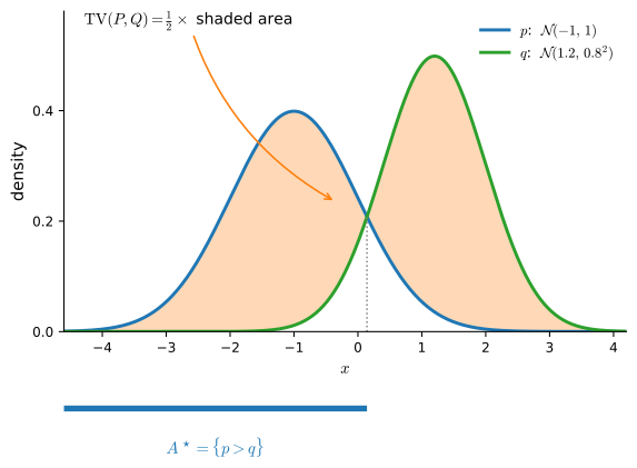
Thus TV bounds what any test can detect. The next inequality says that KL bounds TV: a small KL divergence certifies indistinguishability against every test.
Proposition (Pinsker’s inequality). (Pinsker 1964)
\[ \textrm{TV}(P, Q) \;\leq\; \sqrt{ \tfrac{1}{2}\, D_{\textrm{KL}}(P\|Q) }. \tag{28.2.7}\]
Proof. Step 1: two outcomes. For \(a, b \in (0, 1)\) let \(d(a\|b) = a \log\frac{a}{b} + (1-a) \log\frac{1-a}{1-b}\) be the KL divergence between coins with heads-probabilities \(a\) and \(b\); their TV distance is \(|a - b|\), so we must show \(d(a\|b) \geq 2(a-b)^2\). Fix \(b\) and let \(h(a) = d(a\|b) - 2(a - b)^2\). Then \(h(b) = 0\), \(h'(b) = 0\), and
\[ h''(a) = \frac{1}{a(1-a)} - 4 \geq 0, \]
since \(a(1-a) \leq \tfrac{1}{4}\). A convex function with value and slope zero at \(a = b\) is non-negative everywhere.
Step 2: reduction to two outcomes. Let \(A^\star = \{p > q\}\), and set \(a = P(A^\star)\), \(b = Q(A^\star)\), so that \(\textrm{TV}(P, Q) = a - b\) by the previous proposition. Merging the outcomes inside \(A^\star\) and inside its complement can only decrease KL, by the log-sum inequality: for non-negative numbers,
\[ \sum_i a_i \log\frac{a_i}{b_i} \geq \big(\sum_i a_i\big) \log \frac{\sum_i a_i}{\sum_i b_i}, \]
itself one application of Jensen to \(t \mapsto t\log t\). Applied separately to the terms in \(A^\star\) and in its complement,
\[ D_{\textrm{KL}}(P\|Q) \;\geq\; d(a\|b) \;\geq\; 2(a - b)^2 = 2\,\textrm{TV}(P, Q)^2, \]
which rearranges to Equation 28.2.7. \(\blacksquare\)
The merging step holds in full generality: coarsening the outcome space cannot increase an f-divergence, and the proof above already contains the general argument.
Remark (data-processing for f-divergences). Passing \(P\) and \(Q\) through any channel \(K\) (any deterministic or random map from \(x\) to \(y\), with output distributions \((pK)(y) = \sum_x K(y \mid x)\, p(x)\) and likewise \(qK\)) can only lose distinguishability:
\[ D_f(PK \,\|\, QK) \;\leq\; D_f(P\|Q). \]
Proof. Since \(\sum_y K(y \mid x) = 1\), \(D_f(P\|Q) = \sum_y \sum_x K(y \mid x)\, q(x)\, f\big(p(x)/q(x)\big)\). For each fixed \(y\), Jensen’s inequality with weights proportional to \(K(y \mid x)\, q(x)\), applied at the points \(p(x)/q(x)\), moves \(f\) outside the inner sum and leaves exactly the \(y\)-th term of \(D_f(PK\|QK)\); summing over \(y\) with \((qK)(y) > 0\) finishes, since terms with \((qK)(y) = 0\) contribute nothing. \(\blacksquare\)
Merging outcomes is the deterministic special case used above, and the data-processing inequality for mutual information is the same principle in its best-known form; Section 28.3 states and proves it. Note also what Pinsker does not say: it has no useful converse. TV is bounded by \(1\) while KL is unbounded, so the bound goes slack for distant pairs (two unit-variance Gaussians \(50\) apart have \(\textrm{TV} \approx 1\) but KL \(= 1250\) nats), and small TV does not imply small KL (a model can assign \(q = 0\) to a rare event and have infinite KL at tiny TV). The following experiment checks both the bound and its tightness: over \(10{,}000\) random pairs of distributions on five outcomes, then on pairs of coins approaching each other, where the binary-case analysis says the ratio should approach \(1\).
rng = np.random.default_rng(0)
worst = 0.0
for _ in range(10000):
    pr, qr = rng.dirichlet(np.ones(5)), rng.dirichlet(np.ones(5))
    tv = 0.5 * np.abs(pr - qr).sum()
    kl_pq = np.sum(pr * np.log(pr / qr))
    worst = max(worst, tv / np.sqrt(0.5 * kl_pq))
print(f'max TV / sqrt(KL/2) over 10,000 random pairs: {worst:.4f}')

for eps in (0.1, 0.01, 0.001):
    pr, qr = np.array([0.5, 0.5]), np.array([0.5 + eps, 0.5 - eps])
    tv = 0.5 * np.abs(pr - qr).sum()
    kl_pq = np.sum(pr * np.log(pr / qr))
    print(f'coins 1/2 vs 1/2+{eps}: TV / sqrt(KL/2) = '
          f'{tv / np.sqrt(0.5 * kl_pq):.6f}')
max TV / sqrt(KL/2) over 10,000 random pairs: 0.9926
coins 1/2 vs 1/2+0.1: TV / sqrt(KL/2) = 0.989881
coins 1/2 vs 1/2+0.01: TV / sqrt(KL/2) = 0.999900
coins 1/2 vs 1/2+0.001: TV / sqrt(KL/2) = 0.999999The ratio \(\textrm{TV}/\sqrt{\textrm{KL}/2}\) never exceeds \(1\) (the worst of \(10{,}000\) random pairs reaches \(0.9926\)), and on nearly-fair coins it climbs to \(0.999999\): the constant \(\tfrac{1}{2}\) is the best possible (Exercise 5), a sharpening due to Csiszár (Csiszár 1967) rather than to Pinsker’s original argument.
28.2.3.2 Integral Probability Metrics and MMD
The definition of total variation takes a supremum of differences over events. Replacing indicator functions of events by an arbitrary class \(\mathcal{F}\) of test functions yields the integral probability metrics (Müller 1997):
\[ \textrm{IPM}_{\mathcal{F}}(P, Q) = \sup_{f \in \mathcal{F}} \,\big( E_{x \sim P}[f(x)] - E_{x \sim Q}[f(x)] \big). \tag{28.2.8}\]
The class \(\mathcal{F}\) is a panel of auditors; the IPM reports the largest discrepancy any auditor in the panel can certify. Three choices of panel give three famous distances: bounded functions \(\mathcal{F} = \{f : \|f\|_\infty \leq \tfrac{1}{2}\}\) recover total variation; 1-Lipschitz functions give the Wasserstein-1 distance (next subsection); and the unit ball of a reproducing kernel Hilbert space gives the maximum mean discrepancy (Gretton et al. 2012). Contrast the structure with Equation 28.2.1: f-divergences integrate a function of the density ratio and need densities; IPMs compare expectations and need only samples.
MMD is the member built for computation. A kernel \(k(x, y)\) is a symmetric, positive-definite similarity function; the standard example is the RBF kernel \(k(x,y) = \exp(-\|x - y\|^2 / (2\ell^2))\), which scores two points by how close they are on the length scale \(\ell\). Every such kernel generates a reproducing kernel Hilbert space (RKHS) \(\mathcal{H}\), a space of functions in which \(k(x, \cdot)\) evaluates: \(f(x) = \langle f, k(x, \cdot) \rangle_{\mathcal{H}}\), the reproducing property. (Kernels and their Hilbert spaces are developed at length in (Schölkopf and Smola 2002); these two facts are all we need.) Every distribution gets a mean embedding \(\mu_P = E_{x \sim P}[k(x, \cdot)] \in \mathcal{H}\), its average feature function; for bounded kernels the embedding exists and expectations commute with inner products, so for \(f\) in the unit ball the reproducing property turns expectations into inner products, \(E_P[f] - E_Q[f] = \langle f, \mu_P - \mu_Q \rangle_{\mathcal{H}}\). The supremum over the unit ball of an inner product against a fixed vector is that vector’s norm, so the IPM collapses to \(\textrm{MMD}(P, Q) = \|\mu_P - \mu_Q\|_{\mathcal{H}}\), and squaring expands the norm into three kernel expectations:
\[ \textrm{MMD}^2(P, Q) = E_{x, x' \sim P}[k(x, x')] + E_{y, y' \sim Q}[k(y, y')] - 2\, E_{x \sim P, y \sim Q}[k(x, y)]. \tag{28.2.9}\]
Within-sample similarity under \(P\), plus within-sample similarity under \(Q\), minus twice the across-sample similarity: if the two samples interleave, the three terms cancel; if they form separate clumps, the within terms beat the across term. Replacing expectations by sample averages gives the standard unbiased estimator (Gretton et al. 2012), computable in a few lines with no optimization and no densities; the estimator excludes the diagonal terms \(k(x_i, x_i)\), whose inclusion would bias the within-sample terms upward. For characteristic kernels (the RBF kernel is one) the embedding \(P \mapsto \mu_P\) is injective, so MMD is a genuine metric: zero only at equality.
def mmd2_unbiased(x, y, ell=1.0):
    """Unbiased MMD^2 with the RBF kernel exp(-(a-b)^2 / (2 ell^2))."""
    k = lambda a, b: np.exp(-(a[:, None] - b[None, :]) ** 2 / (2 * ell ** 2))
    kxx, kyy, kxy = k(x, x), k(y, y), k(x, y)
    n, m = len(x), len(y)
    return ((kxx.sum() - np.trace(kxx)) / (n * (n - 1))
            + (kyy.sum() - np.trace(kyy)) / (m * (m - 1))
            - 2 * kxy.mean())

rng = np.random.default_rng(3)
n = 250
x1, y_same = rng.standard_normal(n), rng.standard_normal(n)
y_shift = rng.standard_normal(n) + 0.5
print(f'MMD^2, same distribution : {mmd2_unbiased(x1, y_same):+.5f}')
print(f'MMD^2, mean shifted 0.5  : {mmd2_unbiased(x1, y_shift):+.5f}')
MMD^2, same distribution : +0.00054
MMD^2, mean shifted 0.5 : +0.05890Two samples from the same standard Gaussian give \(\textrm{MMD}^2 \approx 0.0005\) (noise around zero; the unbiased estimator is even allowed to go slightly negative), while shifting one sample’s mean by half a standard deviation produces \(\approx 0.059\), two orders of magnitude larger and, up to sampling noise at \(n = 250\), consistent with the population value \(\approx 0.047\) that Exercise 8 derives in closed form. This sample-only, optimization-free property is why MMD powers kernel two-sample tests and adversary-free generative training (MMD-GANs and generative moment matching (Li et al. 2017; Li et al. 2015)): the “critic” is the whole RKHS ball at once, and Equation 28.2.9 evaluates its supremum in closed form.
28.2.3.3 Optimal Transport and the Wasserstein Distance
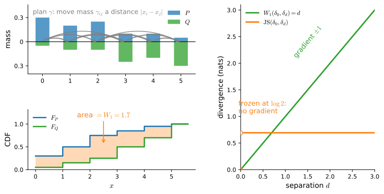
Every divergence so far has a common limitation. Let \(P = \delta_0\) be a point mass at the origin and \(Q_d = \delta_d\) a point mass at distance \(d\). For any \(d \neq 0\) the supports are disjoint, so the density ratio is degenerate everywhere and every f-divergence is a constant: \(D_{\textrm{KL}} = \infty\), \(\textrm{TV} = 1\), \(\textrm{JS} = \log 2\), whether \(d = 0.01\) or \(d = 100\). A generator early in training is in exactly this situation (its samples and the data occupy disjoint slivers of image space), and an objective that is constant in the generator’s parameters supplies zero gradient. This is the vanishing-gradient pathology of GAN training, and it is a property of the divergence, not of the optimizer (Arjovsky et al. 2017).
Geometry still distinguishes distributions with disjoint supports: \(\delta_{0.01}\) is near \(\delta_0\) because mass need only move \(0.01\). The Wasserstein-1 distance (earth-mover’s distance) makes this precise. A coupling \(\gamma\) of \(P\) and \(Q\) is a joint distribution over pairs \((x, y)\) with marginals \(P\) and \(Q\) (a transport plan specifying how much mass travels from each source to each destination, as in Figure 28.2.5), and
\[ W_1(P, Q) = \inf_{\gamma \in \Pi(P, Q)} E_{(x, y) \sim \gamma}\big[ \|x - y\| \big], \tag{28.2.10}\]
the cheapest total mass-times-distance over all plans, for \(P\) and \(Q\) with finite first moments (without that hypothesis the infimum may be infinite). On the point masses, \(W_1(\delta_0, \delta_d) = |d|\): smooth in \(d\), gradient \(\pm 1\), exactly the training signal the f-divergences withheld.
The primal Equation 28.2.10 is an optimization over joint distributions, hard to even parameterize from samples. Its dual is the reason \(W_1\) matters to deep learning.
Proposition (Kantorovich–Rubinstein duality).
\[ W_1(P, Q) = \sup_{\|f\|_{\textrm{Lip}} \leq 1} \big( E_{x \sim P}[f(x)] - E_{y \sim Q}[f(y)] \big), \tag{28.2.11}\]
where the supremum runs over all 1-Lipschitz functions (\(|f(x) - f(y)| \leq \|x - y\|\) for all \(x, y\)).
We do not prove the general statement; see Peyré and Cuturi (2019) . Weak duality is immediate. For any 1-Lipschitz \(f\) and any coupling \(\pi\) of \(P\) and \(Q\), \(f(x)-f(y)\leq \lVert x-y\rVert\). Taking the expectation under \(\pi\) gives \(E_P[f]-E_Q[f]\leq E_\pi[\lVert x-y\rVert]\). The inequality holds for every coupling and every admissible \(f\), hence the dual supremum cannot exceed the primal infimum (compare Section 26.4.4). Kantorovich–Rubinstein duality states that equality is attainable under the usual conditions. Thus \(W_1\) is the 1-Lipschitz IPM: the test class in Equation 28.2.8 consists of functions with slope at most \(1\). The WGAN (Arjovsky et al. 2017) trains exactly this dual: a neural critic plays the role of \(f\), constrained to be (approximately) 1-Lipschitz, by weight clipping originally, then by gradient penalties (Gulrajani et al. 2017) (penalizing \(\|\nabla f\| \neq 1\), since an optimal Kantorovich potential has unit slope along transport rays) and by spectral normalization (Miyato et al. 2018), which caps each layer’s Lipschitz constant through its largest singular value (Section 24.3).
In one dimension, optimal transport collapses to a formula with no optimization left in it.
Proposition (1-D Wasserstein in closed form). For distributions on \(\mathbb{R}\) with CDFs \(F_P\) and \(F_Q\) and finite first moments, granting the duality Equation 28.2.11,
\[ W_1(P, Q) = \int_{-\infty}^{\infty} \lvert F_P(t) - F_Q(t) \rvert \, dt. \tag{28.2.12}\]
Proof. Let \(f\) be 1-Lipschitz; then \(f\) is absolutely continuous with \(|f'(t)| \leq 1\) wherever the derivative exists, and \(f(x) = f(0) + \int_0^x f'(t)\, dt\), a standard fact of real analysis (Folland 1999) that we grant. The constant \(f(0)\) cancels in \(E_P[f] - E_Q[f]\). For \(X \sim P\), writing the inner integral with indicators, \(\int_0^X f'(t)\,dt = \int_0^{\infty} f'(t)\, \mathbf{1}[X > t]\, dt - \int_{-\infty}^0 f'(t)\, \mathbf{1}[X \leq t]\, dt\), and swapping expectation and integral (Fubini’s theorem from Section 25.4, justified by the moment assumption),
\[ E_P\!\left[ \int_0^X f'(t)\, dt \right] = \int_0^{\infty} f'(t)\,(1 - F_P(t))\, dt - \int_{-\infty}^0 f'(t)\, F_P(t)\, dt. \]
Subtracting the same expression for \(Q\), the constants cancel and both pieces merge into one integral over all of \(\mathbb{R}\):
\[ E_P[f] - E_Q[f] = \int_{-\infty}^{\infty} f'(t)\, \big( F_Q(t) - F_P(t) \big)\, dt \;\leq\; \int_{-\infty}^{\infty} \lvert F_P(t) - F_Q(t) \rvert\, dt, \]
using \(|f'| \leq 1\). Equality is attained by integrating the choice \(f'(t) = \mathrm{sign}\big(F_Q(t) - F_P(t)\big)\), which defines a 1-Lipschitz function. By Kantorovich–Rubinstein Equation 28.2.11 the supremum of the left side over 1-Lipschitz \(f\) is \(W_1\), proving Equation 28.2.12. \(\blacksquare\)
Geometrically, \(W_1\) is the area between the two CDFs (the shaded region of Figure 28.2.5). Slicing that area horizontally instead of vertically gives the equivalent quantile form \(W_1 = \int_0^1 |F_P^{-1}(u) - F_Q^{-1}(u)|\, du\), which for two equal-size empirical samples is the mean absolute difference of their sorted values (Exercise 7). The following example compares Equation 28.2.12 with the primal Equation 28.2.10, solved exactly as a linear program over transport plans (the plan \(\gamma\) is a matrix with row sums \(p\) and column sums \(q\), compare Section 26.4.4).
atoms = np.array([0.0, 1.0, 2.0, 3.0, 4.0, 5.0])
p_w = np.array([0.30, 0.20, 0.25, 0.10, 0.10, 0.05])
q_w = np.array([0.05, 0.10, 0.10, 0.25, 0.20, 0.30])

F_p, F_q = np.cumsum(p_w), np.cumsum(q_w)
w1_cdf = np.sum(np.abs(F_p - F_q)[:-1] * np.diff(atoms))

C = np.abs(atoms[:, None] - atoms[None, :])      # cost matrix |x_i - y_j|
k = len(atoms)
A_eq = np.zeros((2 * k, k * k))
for i in range(k):
    A_eq[i, i * k:(i + 1) * k] = 1               # row sums    = p
    A_eq[k + i, i::k] = 1                        # column sums = q
res = optimize.linprog(C.ravel(), A_eq=A_eq,
                       b_eq=np.concatenate([p_w, q_w]), method='highs')
print(f'W1 via the CDF formula : {w1_cdf:.10f}')
print(f'W1 via the primal LP   : {res.fun:.10f}')
W1 via the CDF formula : 1.7000000000
W1 via the primal LP : 1.7000000000Both routes give \(W_1 = 1.7\) to ten decimal places: a one-line integral of CDFs replaces a \(36\)-variable linear program.
Beyond one dimension no such formula exists, and the LP scales poorly: with \(n\) atoms a side it has \(n^2\) variables. The standard fix at scale is entropic regularization (Cuturi 2013): add \(-\varepsilon H(\gamma)\) to the primal objective, penalizing low-entropy (overly deterministic) plans. The regularized problem is strictly convex and its solution has the form \(\gamma = \mathrm{diag}(u)\, K\, \mathrm{diag}(v)\) with \(K = e^{-C/\varepsilon}\), where the Sinkhorn iterations (alternately rescaling rows to match \(p\) and columns to match \(q\)) converge fast, run on matrix-vector products (GPU-friendly), and are differentiable end to end. As \(\varepsilon \to 0\) the entropic cost recovers the unregularized optimum (Peyré and Cuturi 2019).
def sinkhorn(p, q, C, eps, iters=5000):
    """Entropic OT by Sinkhorn iterations; returns plan and cost."""
    K = np.exp(-C / eps)
    u = np.ones_like(p)
    for _ in range(iters):
        v = q / (K.T @ u)
        u = p / (K @ v)
    plan = u[:, None] * K * v[None, :]
    return plan, np.sum(plan * C)

fig, axes = d2l.plt.subplots(1, 3, figsize=(9, 2.8))
axes[0].set_ylabel('source $i$')
for ax, eps in zip(axes, (1.0, 0.1, 0.02)):
    plan, cost = sinkhorn(p_w, q_w, C, eps)
    print(f'epsilon = {eps:4.2f}: entropic cost = {cost:.4f}'
          f'   (unregularized LP: {res.fun:.4f})')
    ax.imshow(plan, cmap='Blues', origin='lower')
    ax.set_title(f'$\\gamma$ at $\\varepsilon = {eps}$')
ax.set_xlabel('destination $j$')epsilon = 1.00: entropic cost = 1.7700 (unregularized LP: 1.7000)
epsilon = 0.10: entropic cost = 1.7000 (unregularized LP: 1.7000)
epsilon = 0.02: entropic cost = 1.7000 (unregularized LP: 1.7000)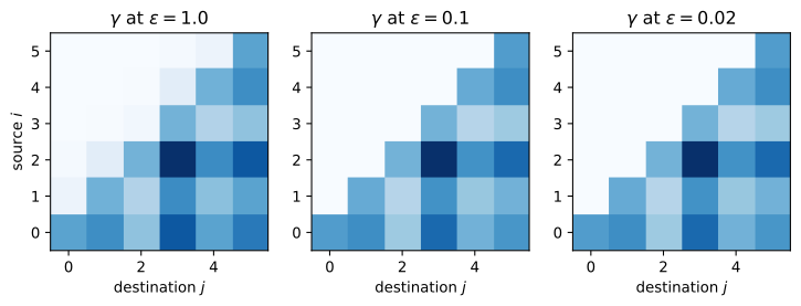
epsilon = 1.00: entropic cost = 1.7700   (unregularized LP: 1.7000)
epsilon = 0.10: entropic cost = 1.7000   (unregularized LP: 1.7000)
epsilon = 0.02: entropic cost = 1.7000   (unregularized LP: 1.7000)
epsilon = 1.00: entropic cost = 1.7700   (unregularized LP: 1.7000)
epsilon = 0.10: entropic cost = 1.7000   (unregularized LP: 1.7000)
epsilon = 0.02: entropic cost = 1.7000   (unregularized LP: 1.7000)
epsilon = 1.00: entropic cost = 1.7700   (unregularized LP: 1.7000)
epsilon = 0.10: entropic cost = 1.7000   (unregularized LP: 1.7000)
epsilon = 0.02: entropic cost = 1.7000   (unregularized LP: 1.7000)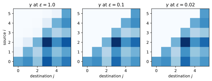
At \(\varepsilon = 1\) the blurred plan costs more (\(1.77\) vs. \(1.70\)); by \(\varepsilon = 0.1\) the entropic cost matches the LP to four decimals. The heatmaps show why. At \(\varepsilon = 1\) entropy dominates and the plan is a haze: every source hedges its mass across many destinations, close to the independent coupling \(p\, q^\top\), so parcels take detours and the cost runs high. Shrinking \(\varepsilon\) anneals the haze away: the plan sharpens toward a vertex of the transport polytope (an extreme point of the set of feasible plans), and at \(\varepsilon = 0.02\) only a thin monotone staircase of routes survives, the never-crossing assignment that one-dimensional optimal transport always produces and the LP finds exactly. With squared cost \(\|x - y\|^2\) in Equation 28.2.10 one obtains the Wasserstein-2 distance, whose dynamical (Benamou–Brenier) formulation as a minimum-kinetic-energy flow is the natural language for diffusion models and flow matching; we develop it where it is needed, in Section 29.4.
28.2.4 Scores: Fisher Divergence, Stein Discrepancy, and the Objective Map
One last family compares distributions through derivatives of their log-densities. Score matching is a principal route that cancels a density’s normalizing constant. It requires differentiable log densities and suitable support or boundary conditions; ratio and Stein methods offer other normalizer-free constructions.
28.2.4.1 The Score and the Fisher Divergence
The score of a distribution \(P\) with differentiable density \(p\) is the gradient of its log-density with respect to the data point:
\[ s_P(\mathbf{x}) = \nabla_{\mathbf{x}} \log p(\mathbf{x}). \tag{28.2.13}\]
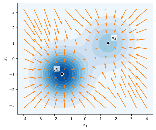
(A terminology hazard: in classical statistics, “score” means the gradient with respect to parameters, \(\nabla_{\boldsymbol{\theta}} \log p_{\boldsymbol{\theta}}(\mathbf{x})\), the object behind maximum likelihood and Fisher information in Section 27.3. Here the gradient is in \(\mathbf{x}\); this data score is the one that Section 29.4 builds diffusion models from.) The score is a vector field on the sample space, pointing in the direction in which the density increases fastest: “uphill, toward where the mass is”, as Figure 28.2.6 shows. For a Gaussian \(\mathcal{N}(\mu, \sigma^2)\) it is
\[ s(x) = -\frac{x - \mu}{\sigma^2}, \]
a spring pulling toward the mean with stiffness \(1/\sigma^2\); for a mixture \(p = \sum_k w_k\, p_k\) the chain rule gives \(s(x) = \sum_k r_k(x)\, s_k(x)\) with \(r_k(x) = w_k p_k(x) / p(x)\): each component’s spring, weighted by the posterior probability (“responsibility”) that \(x\) came from it.
The score is useful because it does not depend on a normalizing constant. Suppose we can only write the density up to a constant, \(p(\mathbf{x}) = \tilde{p}(\mathbf{x}) / Z\) with \(Z = \int \tilde{p}\) intractable, as commonly occurs for energy-based models. Then
\[ \nabla_{\mathbf{x}} \log p(\mathbf{x}) = \nabla_{\mathbf{x}} \log \tilde{p}(\mathbf{x}) - \nabla_{\mathbf{x}} \log Z = \nabla_{\mathbf{x}} \log \tilde{p}(\mathbf{x}), \]
since \(Z\) does not depend on \(\mathbf{x}\). The score never sees the normalizer. A divergence built from scores therefore lets us fit unnormalized models, and the natural choice is the mean squared mismatch of the two vector fields under the data distribution, the Fisher divergence:
\[ D_{\textrm{F}}(P\|Q) = \frac{1}{2}\, E_{\mathbf{x} \sim P}\!\left[ \big\| \nabla_{\mathbf{x}} \log p(\mathbf{x}) - \nabla_{\mathbf{x}} \log q(\mathbf{x}) \big\|^2 \right]. \tag{28.2.14}\]
It is non-negative. If \(p\) and \(q\) are positive on the same connected support, score equality \(P\)-almost everywhere forces \(\log p-\log q\) to be constant there, and normalization then gives \(P=Q\). Connected support of \(P\) alone is not enough: \(Q\) could agree with \(P\) on that support while assigning additional mass elsewhere. For two equal-variance Gaussians the scores differ by the constant \((\mu_2 - \mu_1)/\sigma^2\), so \(D_{\textrm{F}} = (\mu_1 - \mu_2)^2 / (2\sigma^4)\); compare KL’s \((\mu_1 - \mu_2)^2/(2\sigma^2)\) from Equation 28.1.5; the general unequal-variance form is Exercise 9. The following example verifies the mixture score formula, the normalizer-blindness, and the Gaussian closed form numerically.
def score_p(x):
    """Score of the mixture P: responsibility-weighted component scores."""
    log_comps = np.stack([np.log(wi) - 0.5 * np.log(2 * np.pi * si ** 2)
                          - (x - mi) ** 2 / (2 * si ** 2)
                          for wi, mi, si in zip(w, mus, sigmas)])
    r = np.exp(log_comps - log_p(x))             # responsibilities r_k(x)
    comp_scores = np.stack([-(x - mi) / si ** 2 for mi, si in zip(mus, sigmas)])
    return np.sum(r * comp_scores, axis=0)

numeric = np.gradient(log_p(x), x)               # numerical d/dx log p
gap = np.abs(score_p(x) - numeric)[10:-10].max()
print(f'mixture score, max |analytic - numerical|: {gap:.2e}')
shifted = np.gradient(np.log(2.7) + log_p(x), x)  # unnormalized: 2.7 * p
print(f'score change from rescaling p by 2.7    : '
      f'{np.abs(shifted - numeric).max():.2e}')

mu1, s1, mu2, s2 = 0.0, 1.0, 1.0, 1.0
xs = np.linspace(-10.0, 12.0, 4001)
pdf1 = np.exp(-(xs - mu1) ** 2 / (2 * s1 ** 2)) / np.sqrt(2 * np.pi * s1 ** 2)
sc1, sc2 = -(xs - mu1) / s1 ** 2, -(xs - mu2) / s2 ** 2
fisher = 0.5 * integrate.trapezoid(pdf1 * (sc1 - sc2) ** 2, xs)
print(f'Fisher divergence N(0,1)||N(1,1): quadrature {fisher:.6f}, '
      f'closed form {(mu1 - mu2) ** 2 / (2 * s1 ** 4):.6f}')
mixture score, max |analytic - numerical|: 3.52e-04
score change from rescaling p by 2.7 : 1.82e-12
Fisher divergence N(0,1)||N(1,1): quadrature 0.500000, closed form 0.500000The analytic mixture score matches the numerical gradient of \(\log p\) to the grid’s finite-difference accuracy (\(\approx 3.5 \times 10^{-4}\)), rescaling the density by \(2.7\) changes the score only at floating-point precision (\(\approx 2 \times 10^{-12}\)), and the quadrature reproduces the Gaussian closed form \(0.5\) to six decimals.
One apparent obstacle remains: Equation 28.2.14 is an expectation involving \(\nabla \log p\) of the data distribution, which we do not know either. The resolution is Hyvärinen’s score matching identity (Hyvärinen 2005), an integration by parts showing that, up to a constant independent of the model,
\[ D_{\textrm{F}}(P\|Q_{\boldsymbol{\theta}}) = E_{\mathbf{x} \sim P}\!\left[ \tfrac{1}{2} \|\mathbf{s}_{\boldsymbol{\theta}}(\mathbf{x})\|^2 + \nabla_{\mathbf{x}} \cdot \mathbf{s}_{\boldsymbol{\theta}}(\mathbf{x}) \right] + \textrm{const}, \]
an objective containing only the model’s score \(\mathbf{s}_{\boldsymbol{\theta}}\), estimable from data samples alone. We state it here and prove it, together with its denoising variant (the actual training loss of diffusion models), in Section 29.4.
28.2.4.2 Stein’s Identity
The score can also test a sample. The starting point is a fact about expectations under a distribution whose score we know.
Proposition (Stein’s identity). (Stein 1981) Let \(P\) have a differentiable density \(p > 0\) on \(\mathbb{R}\) with score \(s_P = (\log p)'\), and let \(f\) be differentiable with \(f(x)\, p(x) \to 0\) as \(x \to \pm\infty\). Then
\[ E_{x \sim P}\big[ f'(x) + f(x)\, s_P(x) \big] = 0. \tag{28.2.15}\]
Proof. Since \(p' = s_P\, p\), integration by parts (Section 25.4.2.2) gives
\[ \int f'(x)\, p(x)\, dx = \big[ f(x)\, p(x) \big]_{-\infty}^{\infty} - \int f(x)\, p'(x)\, dx = 0 - \int f(x)\, s_P(x)\, p(x)\, dx, \]
and moving the right-hand side over is Equation 28.2.15. \(\blacksquare\)
For \(P = \mathcal{N}(0, 1)\) the score is \(s_P(x) = -x\) and the identity reads \(E[f'(X)] = E[X f(X)]\); with \(f(x) = x\) it recovers \(E[X^2] = 1\). The point is that the identity holds for huge classes of \(f\) simultaneously, and only for \(P\) itself: if a sample’s averages violate Equation 28.2.15 for some \(f\), the sample is not from \(P\). A Monte-Carlo check of Equation 28.2.15:
rng = np.random.default_rng(7)
z = rng.standard_normal(1_000_000)
# Stein operator for P = N(0,1):  (A_P f)(x) = f'(x) - x f(x)
for name, f, fprime in [('x^3', lambda t: t ** 3, lambda t: 3 * t ** 2),
                        ('sin x', np.sin, np.cos)]:
    val = (fprime(z) - z * f(z)).mean()
    print(f"E[ f'(Z) - Z f(Z) ] for f(x) = {name}: {val:+.4f}")
E[ f'(Z) - Z f(Z) ] for f(x) = x^3: +0.0020
E[ f'(Z) - Z f(Z) ] for f(x) = sin x: +0.0005Both averages (\(+0.0020\) and \(+0.0005\) on a million samples) are zero to within Monte-Carlo error, for two quite different test functions, a glimpse of the infinite family of constraints the identity imposes.
28.2.4.3 The Kernel Stein Discrepancy
To turn the identity into a divergence, run the IPM construction of Section 28.2.3.2 on it: apply the Stein operator \((\mathcal{A}_P f)(x) = f'(x) + f(x)\, s_P(x)\) to every \(f\) in the unit ball of an RKHS and take the largest violation, \(\sup_{\|f\|_{\mathcal{H}} \leq 1} E_{x \sim Q}[(\mathcal{A}_P f)(x)]\). By Stein’s identity the supremum is zero when \(Q = P\); when \(Q \neq P\), some test function witnesses the mismatch. Exactly as with MMD, the supremum over an RKHS ball has a closed form: it is the square root of an expected kernel. For a positive-definite kernel \(k\) and score \(s_P = \nabla \log p\), define the Stein kernel of \(P\),
\[ \begin{aligned} u_P(\mathbf{x}, \mathbf{x}') = {}& s_P(\mathbf{x})^\top k(\mathbf{x}, \mathbf{x}')\, s_P(\mathbf{x}') + s_P(\mathbf{x})^\top \nabla_{\mathbf{x}'} k(\mathbf{x}, \mathbf{x}') \\ &+ \nabla_{\mathbf{x}} k(\mathbf{x}, \mathbf{x}')^\top s_P(\mathbf{x}') + \nabla_{\mathbf{x}} \cdot \nabla_{\mathbf{x}'} k(\mathbf{x}, \mathbf{x}'), \end{aligned} \tag{28.2.16}\]
where the last term is the sum of mixed partials \(\sum_i \partial_{x_i} \partial_{x'_i} k\); in one dimension it reduces to \(\partial_x \partial_{x'} k\). The squared kernel Stein discrepancy (KSD) is the expected Stein kernel under two independent draws from \(Q\):
\[ \mathrm{KSD}^2(Q, P) = E_{\mathbf{x}, \mathbf{x}' \sim Q}\big[ u_P(\mathbf{x}, \mathbf{x}') \big]. \tag{28.2.17}\]
Three properties make KSD useful for modern models. First, Equation 28.2.16 involves \(P\) only through its score, so by the normalizer-blindness of Section 28.2.4.1 an unnormalized model works exactly as well as a normalized one, and no samples from \(P\) are ever drawn. Second, for suitable kernels (the RBF kernel among them, under mild conditions on the score) \(\mathrm{KSD}^2(Q, P) = 0\) if and only if \(Q = P\) (Liu et al. 2016; Chwialkowski et al. 2016). Third, Equation 28.2.17 is a double expectation under \(Q\) alone, so a sample \(x_1, \ldots, x_n \sim Q\) gives the unbiased U-statistic estimator
\[ \widehat{\mathrm{KSD}}^2 = \frac{1}{n(n-1)} \sum_{i \neq j} u_P(x_i, x_j), \]
the same diagonal-excluding average as the MMD estimator. The following example computes it. For the 1-D RBF kernel \(k(x, y) = e^{-(x-y)^2/(2\ell^2)}\) the derivatives in Equation 28.2.16 are closed-form: \(\partial_y k = \frac{x-y}{\ell^2}\, k\), \(\partial_x k = -\frac{x-y}{\ell^2}\, k\), and \(\partial_x \partial_y k = \big( \frac{1}{\ell^2} - \frac{(x-y)^2}{\ell^4} \big)\, k\). We test one sample from \(Q = \mathcal{N}(0, 1)\) against two models: the true \(P = \mathcal{N}(0, 1)\), whose score is \(s(x) = -x\), and the wrong \(P' = \mathcal{N}(1, 1)\), whose score is \(s(x) = -(x - 1)\).
def ksd2_ustat(x, score, ell=1.0):
    """U-statistic KSD^2 with the RBF kernel exp(-(a-b)^2 / (2 ell^2))."""
    d = x[:, None] - x[None, :]
    k = np.exp(-d ** 2 / (2 * ell ** 2))
    dk_dx = -d / ell ** 2 * k
    dk_dy = d / ell ** 2 * k
    d2k = (1 / ell ** 2 - d ** 2 / ell ** 4) * k
    s = score(x)
    u = (s[:, None] * s[None, :] * k + s[:, None] * dk_dy
         + dk_dx * s[None, :] + d2k)
    n = len(x)
    return (u.sum() - np.trace(u)) / (n * (n - 1))

rng = np.random.default_rng(1)
x_q = rng.standard_normal(1000)          # the sample: Q = N(0, 1)
for name, s in [('true model  N(0,1)', lambda t: -t),
                ('wrong model N(1,1)', lambda t: -(t - 1))]:
    print(f'KSD^2 vs the {name}: {ksd2_ustat(x_q, s):+.5f}')
KSD^2 vs the true model N(0,1): +0.00019
KSD^2 vs the wrong model N(1,1): +0.64425Against the true model the U-statistic is \(\approx 0.0002\), consistent with zero (like the unbiased MMD estimator, it may even dip slightly negative); against the model whose mean is off by one it is \(\approx 0.64\): positive and three orders of magnitude larger, although the sample never changed and \(P'\) was never sampled at all: the discrepancy reads the mismatch straight off the score. This sample-versus-model comparison makes KSD the natural goodness-of-fit test for unnormalized models (Liu et al. 2016), and the descent direction it induces on a particle set is Stein variational gradient descent (SVGD) (Liu and Wang 2016), which transports particles toward \(P\) using only its score.
28.2.4.4 The Divergence-to-Objective Map
The table records idealized population correspondences. Exact equalities may require an unrestricted optimal critic, a sufficiently rich model family, and population expectations. A restricted critic, finite data, and incomplete optimization can change both the effective objective and its behavior.
| Training objective | Idealized divergence | Treated in | Tendency and qualification |
|---|---|---|---|
| maximum likelihood: autoregressive models, normalizing flows | forward KL | Section 28.2.2.2 | penalizes assigning zero density to data; model constraints govern coverage |
| variational inference, VAE posterior (ELBO) | reverse KL | Section 28.2.2.2 | may select one mode in restricted families; local optima also matter |
| original GAN with optimal discriminator | Jensen–Shannon | Section 28.2.2.1 | the ideal objective saturates on disjoint supports |
| f-GAN with unrestricted optimal critic | chosen f-divergence | Section 28.2.2.1 | a restricted or underoptimized critic gives only a lower bound |
| WGAN with a valid optimal Lipschitz critic | Wasserstein-1 | Section 28.2.3.3 | measures displacement across disjoint supports; critic enforcement is approximate |
| MMD-GAN, two-sample tests | MMD | Section 28.2.3.2 | closed-form, adversary-free; kernel choice sets sensitivity |
| score matching, diffusion models | Fisher divergence | Section 28.2.4.1 | normalizer-free; trains on the score field |
| SVGD, model criticism | kernel Stein discrepancy | Section 28.2.4.2 | needs only the model’s score; no model samples |
Maximum likelihood (row 1) is forward KL by the NLL–cross-entropy equivalence of Section 27.3.2.1, so a language model trained on next-token prediction is penalized heavily for assigning negligible probability to observed text. Whether it covers all relevant modes depends on model capacity, data, and optimization. In the ideal-discriminator analysis, the original GAN’s bounded divergence saturates on disjoint supports; WGAN instead optimizes a transport dual with a Lipschitz critic, whose approximation determines the usable gradient. Diffusion models compare score fields: the normalizer cancels, and the training loss becomes a regression onto \(\nabla_{\mathbf{x}}\log p\), where Section 29.4 develops the corresponding models.
The divergence supplies one inductive bias. Model restriction, critic class, sampling, and optimization determine how strongly the idealized tendency appears.
28.2.5 Summary
- A divergence demands only \(D(P, Q) \geq 0\) with equality iff \(P = Q\); metrics add symmetry and the triangle inequality. KL is a divergence but not a metric; TV, Hellinger, and Wasserstein are metrics.
- f-divergences \(D_f(P\|Q) = E_Q[f(p/q)]\) unify KL, reverse KL, \(\chi^2\), Hellinger, TV, and Jensen–Shannon; non-negativity is Jensen’s inequality, and near \(P = Q\) all smooth members agree up to the factor \(f''(1)\). The Rényi/\(\alpha\) family sweeps between the two KL directions with a single knob and appears in differential-privacy accounting.
- Fenchel duality turns any f-divergence into an adversarial game, \(D_f = \sup_T \{ E_P[T] - E_Q[f^*(T)] \}\), estimable from samples; the original GAN is the Jensen–Shannon case, and an undertrained critic biases the estimate low.
- The direction of KL is a modeling decision: forward KL (maximum likelihood) is zero-avoiding and mass-covering; reverse KL (variational inference) is zero-forcing and often mode-seeking on multimodal targets; the number and location of local optima depend on the model family.
- Total variation is the largest probability any event can disagree by, and Pinsker’s inequality \(\textrm{TV} \leq \sqrt{D_{\textrm{KL}}/2}\) means small KL certifies indistinguishability under every test.
- IPMs replace events by a test-function class; the RKHS ball gives MMD, with a closed-form unbiased estimator from samples alone.
- Wasserstein distances measure mass transport and remain informative and continuous when supports are disjoint (they need not be differentiable or smooth there), equal an integral of CDF differences in 1-D, and are computed at scale by entropic regularization and Sinkhorn iterations.
- The score \(\nabla_{\mathbf{x}} \log p\) does not depend on the normalizing constant; the Fisher divergence compares score fields and underlies score matching and diffusion; Stein’s identity and the kernel Stein discrepancy turn the score into goodness-of-fit tests.
28.2.6 Exercises
Recover KL and reverse KL from the template Equation 28.2.1 with the generators \(f(u) = u \log u\) and \(f(u) = -\log u\). Then show that for any constant \(c\), the generators \(f(u)\) and \(f(u) + c\,(u - 1)\) define the same divergence, and use this freedom to find a generator for reverse KL that is non-negative everywhere.
Derive the convex conjugate \(f^*(t) = t + t^2/4\) of the \(\chi^2\) generator \(f(u) = (u - 1)^2\) over \(u \in \mathbb{R}\), then redo the computation over the generator’s true domain \(u \in (0, \infty)\) and show that the supremum is \(t + t^2/4\) for \(t \geq -2\) but \(-1\) for \(t \leq -2\). Explain why plugging the (larger) \(\mathbb{R}\)-conjugate into Equation 28.2.5 still yields a valid lower bound, merely a weaker one for critics that dip below \(-2\). Finally, write the explicit f-GAN objective for this generator and verify that the critic \(T^\star = f'(p/q) = 2(p/q - 1)\) attains the bound with equality.
Two point masses at distance \(d\): show that \(D_{\textrm{KL}}\), TV, and JS are constant in \(d\) (for \(d \neq 0\)) while \(W_1 = |d|\). What does this imply about the gradient each objective supplies to a generator whose samples are far from the data?
Prove that total variation satisfies the triangle inequality, and decide which of KL, reverse KL, squared Hellinger, and \(W_1\) are metrics. (For the Hellinger distance \(H = \sqrt{H^2}\), relate it to an \(\ell_2\) norm of \(\sqrt{p} - \sqrt{q}\).)
Sharpness of Pinsker: for coins with biases \(\tfrac{1}{2}\) and \(\tfrac{1}{2} + \epsilon\), expand the KL divergence to second order in \(\epsilon\) to show \(D_{\textrm{KL}} = 2\epsilon^2 + O(\epsilon^4)\) and conclude that the ratio \(\textrm{TV}/\sqrt{D_{\textrm{KL}}/2}\) tends to \(1\), matching the experiment. Why is the bound loose for two unit-variance Gaussians with distant means?
Hellinger and total variation control each other. With the squared Hellinger divergence of the gallery, \(H^2(P, Q) = \sum_x \big(\sqrt{p(x)} - \sqrt{q(x)}\big)^2\), and \(H = \sqrt{H^2}\) the Hellinger distance, prove the two-sided bound
\[ \tfrac{1}{2}\, H^2(P, Q) \;\leq\; \textrm{TV}(P, Q) \;\leq\; H(P, Q)\, \sqrt{ 1 - \tfrac{1}{4} H^2(P, Q) }. \]
(Hint: write \(|p - q| = |\sqrt{p} - \sqrt{q}|\,(\sqrt{p} + \sqrt{q})\). The lower bound is \(\sqrt{p} + \sqrt{q} \geq |\sqrt{p} - \sqrt{q}|\); the upper bound is Cauchy–Schwarz
- together with \(\sum_x (\sqrt{p} + \sqrt{q})^2 = 4 - H^2\).) Then verify both inequalities numerically over \(10{,}000\) random Dirichlet pairs on five outcomes, in the style of the Pinsker experiment, and record how close each side comes to equality. Unlike Pinsker, this sandwich is two-sided: Hellinger and TV agree about which sequences of distributions converge, whereas KL can be infinite at arbitrarily small TV.
From Equation 28.2.12, derive the quantile form \(W_1 = \int_0^1 |F_P^{-1}(u) - F_Q^{-1}(u)|\, du\), and show that for two empirical distributions on samples \(x_1, \ldots, x_n\) and \(y_1, \ldots, y_n\) it equals \(\tfrac{1}{n}\sum_i |x_{(i)} - y_{(i)}|\), the mean absolute difference of sorted values. Verify numerically against the linear program on a small example.
For \(P = \mathcal{N}(0, 1)\) and \(Q = \mathcal{N}(\delta, 1)\) with the RBF kernel of bandwidth \(\ell = 1\), use the Gaussian integral \(E[e^{-Z^2/2}] = (1 + s^2)^{-1/2} e^{-m^2/(2(1+s^2))}\) for \(Z \sim \mathcal{N}(m, s^2)\) to derive \(\textrm{MMD}^2 = \tfrac{2}{\sqrt{3}}\big(1 - e^{-\delta^2/6}\big)\). Evaluate it at \(\delta = 0.5\) and compare with the estimate from the code cell.
Compute the Fisher divergence between \(\mathcal{N}(\mu_1, \sigma_1^2)\) and \(\mathcal{N}(\mu_2, \sigma_2^2)\) in closed form (the score difference is affine in \(x\), so only Gaussian first and second moments are needed), and check it reduces to \((\mu_1 - \mu_2)^2/(2\sigma^4)\) for equal variances. Then verify Stein’s identity Equation 28.2.15 for \(\mathcal{N}(0, 1)\) with \(f(x) = x\) by hand. What classical fact about the standard Gaussian do you recover?