%matplotlib inline
import math
import numpy as np
from d2l import torch as d2l2.6 Generalization
A model is trained on a finite collection of examples, but it is usually deployed on examples it has not seen. A small training error therefore does not by itself establish that the model has learned a useful pattern: a model may instead have fit details specific to its training set.
The central question is how well the fitted model predicts data drawn from the same population but not used for fitting. This distinction matters whenever predictions concern future observations, new patients, or other unseen cases. This is the statistical problem of generalization: determining whether patterns fitted on a sample apply to new observations from the same population.
In real life, we must fit our models using a finite collection of data. The typical scales of that data vary wildly across domains. For many important medical problems, we can only access a few thousand data points. When studying rare diseases, we might be lucky to access hundreds. By contrast, the largest public datasets consisting of labeled photographs, e.g., ImageNet (Deng et al. 2009), contain millions of images. And some unlabeled image collections such as the Flickr YFC100M dataset can be even larger, containing over 100 million images (Thomee et al. 2016). However, even at this extreme scale, the number of available data points remains tiny relative to the space of all possible images at a megapixel resolution. Whenever we work with finite samples, we must keep in mind the risk that we might fit our training data, only to find that the fitted pattern does not generalize.
The phenomenon of fitting closer to our training data than to the underlying distribution is called overfitting, and techniques for combatting overfitting are often called regularization methods. This section develops the intuition needed for the subsequent experiments. Section 3.6 gives a first, rigorous taste; see also Vapnik (1998); Boucheron et al. (2005). We will revisit generalization in many chapters throughout the book, exploring both what is known about the principles underlying generalization in various models, and also heuristic techniques that have been found (empirically) to yield improved generalization on tasks of practical interest.
2.6.1 Training Error and Generalization Error
In the standard supervised learning setting, we assume that the training data and the test data are drawn independently from identical distributions. This is commonly called the IID assumption. Without assumptions relating the training and test distributions, observations from \(P(X,Y)\) do not by themselves determine performance on \(Q(X,Y)\). Making such leaps turns out to require strong assumptions about how \(P\) and \(Q\) are related. Later on we will discuss some assumptions that allow for shifts in distribution but first we need to understand the IID case, where \(P(\cdot) = Q(\cdot)\).
To begin with, we need to differentiate between the training error \(R_\textrm{emp}\), which is a statistic calculated on the training dataset, and the generalization error \(R\), which is an expectation taken with respect to the underlying distribution. You can think of the generalization error as what you would see if you applied your model to an infinite stream of additional data examples drawn from the same underlying data distribution. Formally the training error is expressed as an average over the finite training sample (with the same notation as Section 2.1):
\[R_\textrm{emp}[\mathbf{X}, \mathbf{y}, f] = \frac{1}{n} \sum_{i=1}^n l(\mathbf{x}^{(i)}, y^{(i)}, f(\mathbf{x}^{(i)})), \tag{2.6.1}\]
while the generalization error (also called the risk) is expressed as an integral:
\[R[P, f] = E_{(\mathbf{x}, y) \sim P} [l(\mathbf{x}, y, f(\mathbf{x}))] = \int \int l(\mathbf{x}, y, f(\mathbf{x})) p(\mathbf{x}, y) \;d\mathbf{x} dy. \tag{2.6.2}\]
In typical applications, we cannot calculate the generalization error \(R\) exactly because the density \(p(\mathbf{x}, y)\) is unavailable. Moreover, we cannot sample an infinite stream of data points. Thus, in practice, we must estimate the generalization error by applying our model to an independent test set constituted of a random selection of examples \(\mathbf{X}'\) and labels \(\mathbf{y}'\) that were withheld from our training set. This consists of applying the same formula that was used for calculating the empirical training error but to a test set \(\mathbf{X}', \mathbf{y}'\).
When we evaluate a model fixed independently of the test set, we are working with a fixed model (it does not depend on the sample of the test set), so estimating its error is a mean-estimation problem. However the same cannot be said for the training set. Note that the model we wind up with depends explicitly on the selection of the training set and thus the training error will in general be a biased estimate of the true error on the underlying population. The central question of generalization is then this: when should we expect our training error to be close to the population error (and thus the generalization error)?
2.6.1.1 Model Complexity
In classical theory, when we have simple models and abundant data, the training and generalization errors tend to be close. However, when we work with more complex models and/or fewer examples, we expect the training error to go down but the generalization gap to grow. That gap is the difference \(R - R_\textrm{emp}\) between the generalization error and the training error. Consider a model class so expressive that for any dataset of \(n\) examples, we can find a set of parameters that can perfectly fit arbitrary labels, even if randomly assigned. In this case, even if we fit our training data perfectly, how can we conclude anything about the generalization error? For all we know, our generalization error might be no better than random guessing.
In general, absent any restriction on our model class, we cannot conclude, based on fitting the training data alone, that our model has discovered any generalizable pattern (Vapnik et al. 1994). On the other hand, if our model class was not capable of fitting arbitrary labels, then low training error is evidence that it has captured a real pattern, provided the sample is large relative to the class’s capacity (Section 27.6). Learning-theoretic ideas about model complexity derived some inspiration from the ideas of Karl Popper, an influential philosopher of science, who formalized the criterion of falsifiability (Popper 2005). Popper argued that a scientific theory must exclude some possible observations. The analogy here is that a hypothesis class able to fit every possible labeling receives little support from training fit alone.
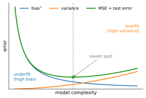
Now what precisely constitutes an appropriate notion of model complexity is a complex matter. For squared-error regression, with expectation taken over repeated training sets drawn by the same process, the classical bias-variance decomposition makes the trade-off precise: a model too simple to capture the signal makes a systematic error (high bias, i.e., underfitting), while a model flexible enough to chase the noise in a particular training set varies wildly from one dataset to the next (high variance, i.e., overfitting). Their sum plus an irreducible noise floor \(\sigma^2\) is the expected test error, which traces the U-shaped curve of Figure 2.6.1; we derive the decomposition formally in Section 27.5. Often, models with more parameters are able to fit a greater number of arbitrarily assigned labels. However, this is not necessarily true. For instance, kernel methods operate in spaces with infinite numbers of parameters, yet their complexity is controlled by other means (Schölkopf and Smola 2002). One notion of complexity that often proves useful is the range of values that the parameters can take. Here, a model whose parameters are permitted to take arbitrary values would be more complex. We will revisit this idea in the next section, when we introduce weight decay, your first practical regularization technique. It can be difficult to compare complexity among members of substantially different model classes (say, decision trees vs. neural networks).
A qualification becomes important for deep neural networks. When a model is capable of fitting arbitrary labels, low training error does not necessarily imply low generalization error. However, it does not necessarily imply high generalization error either. All we can say with confidence is that low training error alone is not enough to certify low generalization error. Deep neural networks can fit arbitrary labels yet often generalize on structured real data. Their training error alone therefore provides limited evidence about generalization. In these cases we must rely more heavily on our holdout data to certify generalization after the fact. Error on the holdout data, i.e., validation set, is called the validation error.
The classical picture says that more capacity (the richness of the model class) means more overfitting. For the heavily overparametrized models used in modern deep learning, however, that picture is incomplete. Once a model is large enough to interpolate its training data (drive training error to zero), pushing capacity even higher often makes test error fall again rather than rise: the double descent phenomenon (Belkin et al. 2019; Nakkiran et al. 2021). We examine this phenomenon and the limits of the classical complexity picture in Section 4.5; for a quantitative treatment that reproduces the double-descent curve from scratch, see Section 27.6.
2.6.2 Underfitting or Overfitting?
When we compare the training and validation errors, two common situations are useful to distinguish. The first occurs when our training error and validation error are both substantial but there is only a small gap between them. If the model is unable to reduce the training error, that could mean that our model is too simple (i.e., insufficiently expressive) to capture the pattern that we are trying to model. Moreover, since the generalization gap between our training and generalization errors is small, we have reason to believe that we could get away with a more complex model. This phenomenon is known as underfitting.
On the other hand, as we discussed above, we want to watch out for the cases when our training error is significantly lower than our validation error, indicating severe overfitting. Note that overfitting is not always a bad thing. In deep learning especially, the best predictive models often perform far better on training data than on holdout data. Ultimately, we usually care about driving the generalization error lower, and only care about the gap insofar as it becomes an obstacle to that end. Note that if the training error is zero, then the generalization gap is precisely equal to the generalization error and we can make progress only by reducing the gap.
2.6.2.1 Polynomial Curve Fitting
To illustrate some classical intuition about overfitting and model complexity, consider the following: given training data consisting of a single feature \(x\) and a corresponding real-valued label \(y\), we try to find the polynomial of degree \(d\)
\[\hat{y}= \sum_{i=0}^d x^i w_i\]
for estimating the label \(y\). This is just a linear regression problem where our features are given by the powers of \(x\), the model’s weights are given by \(w_i\), and the bias is given by \(w_0\) since \(x^0 = 1\) for all \(x\). Since this is just a linear regression problem, we can use the squared error as our loss function.
A higher-order polynomial function is more complex than a lower-order polynomial function, since the higher-order polynomial has more parameters and the model function’s selection range is wider. Fixing the training dataset, higher-order polynomial functions should always achieve lower (at worst, equal) training error relative to lower-degree polynomials. In fact, whenever each data example has a distinct value of \(x\), a polynomial function with degree at most one less than the number of data examples can fit the training set perfectly. We compare the relationship between polynomial degree (model complexity) and both underfitting and overfitting in Figure 2.6.1.
To demonstrate this behavior, we generate data from a known cubic and fit polynomials of growing degree to a small training set.
%matplotlib inline
import math
import numpy as np
from d2l import tensorflow as d2l%matplotlib inline
import math
import numpy as np
from d2l import jax as d2l%matplotlib inline
import math
import numpy as np
from d2l import mxnet as d2lWe draw inputs \(x\) uniformly from \([-1, 1]\), build a design matrix whose \(i\)-th column is \(x^i\), and generate labels from a degree-3 target \(y = 5 + 1.2 x - 3.4 x^2 + 5.6 x^3\) plus a little Gaussian noise. We deliberately keep the training set small so that high-degree models have room to overfit.
np.random.seed(0)
max_degree = 20                  # highest polynomial degree we will fit
n_train, n_test = 20, 100        # few training points, so high degrees overfit
true_w = np.zeros(max_degree)
true_w[:4] = np.array([5, 1.2, -3.4, 5.6])

x = np.random.uniform(-1, 1, size=n_train + n_test)
poly = np.power(x.reshape(-1, 1), np.arange(max_degree))   # column i holds x**i
labels = poly @ true_w + np.random.normal(scale=0.1, size=n_train + n_test)
Fitting the first \(d+1\) columns by least squares gives the best degree-\(d\) polynomial; we record its loss on both the training and the held-out test split.
def fit_degree(d):
    cols = slice(0, d + 1)
    w, *_ = np.linalg.lstsq(poly[:n_train, cols], labels[:n_train], rcond=None)
    err = poly[:, cols] @ w - labels
    return (err[:n_train] ** 2).mean(), (err[n_train:] ** 2).mean()
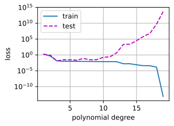
A degree-1 polynomial is too rigid to capture a cubic, so it errs on both splits (underfitting); degree 3 matches the true model, with low error on both; and a degree-19 polynomial has enough freedom to interpolate the 20 training points almost exactly, driving training error toward zero while test error explodes (overfitting).
for name, d in [('underfitting (degree 1) ', 1),
                ('just right   (degree 3) ', 3),
                ('overfitting   (degree 19)', 19)]:
    train_mse, test_mse = fit_degree(d)
    print(f'{name}: train {train_mse:8.4f}   test {test_mse:12.4f}')
underfitting (degree 1) : train 1.6698 test 1.7318
just right (degree 3) : train 0.0136 test 0.0129
overfitting (degree 19): train 0.0000 test 49271508224071.6328For this seeded dataset, sweeping the degree from 1 to 19 produces the U-shaped test-error pattern sketched in Figure 2.6.1: error first falls as the model gains the capacity to represent the signal, then rises as the surplus capacity is spent fitting noise. Training error, by contrast, only ever decreases.
degrees = list(range(1, max_degree))
mse = np.array([fit_degree(d) for d in degrees])
d2l.plot(degrees, [mse[:, 0], mse[:, 1]], xlabel='polynomial degree',
         ylabel='loss', legend=['train', 'test'], yscale='log')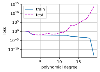
Because the data generator is known, the experiment can estimate bias and variance separately. Because we know the noiseless target \(f(x) = 5 + 1.2 x - 3.4 x^2 + 5.6 x^3\), we can redraw the training noise many times, refit the degree-\(d\) polynomial on each draw, and ask two questions on the held-out inputs: how far is the average fit from the truth (squared bias), and how much does the fit fluctuate across draws (variance)?
f = poly @ true_w                        # noiseless target on all inputs
bias2, var = [], []
for d in range(1, 15):
    preds = []
    for _ in range(200):                 # 200 fresh draws of training noise
        y_tr = f[:n_train] + np.random.normal(scale=0.1, size=n_train)
        w, *_ = np.linalg.lstsq(poly[:n_train, :d+1], y_tr, rcond=None)
        preds.append(poly[n_train:, :d+1] @ w)
    preds = np.stack(preds)
    bias2.append(((preds.mean(0) - f[n_train:]) ** 2).mean())
    var.append(preds.var(0).mean())
d2l.plot(list(range(1, 15)), [bias2, var, np.array(bias2) + np.array(var)],
         xlabel='polynomial degree', ylabel='error', yscale='log',
         legend=['bias^2', 'variance', 'bias^2 + variance'])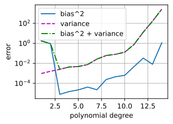
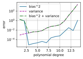
The estimated curve now separates into its two components. For these inputs and 200 noise redraws, squared bias becomes small once the model class contains the cubic target, while variance rises sharply at high degrees. Their sum is smallest near degree 3. Up to the irreducible noise floor \(\sigma^2 = 0.01\), the population bias–variance decomposition identifies this sum with expected test error; the plotted quantities are Monte Carlo estimates of its terms. This is a numerical instance of the decomposition proved in Section 27.5.
2.6.2.2 Dataset Size
Beyond model complexity, another big consideration to bear in mind is dataset size. Fixing our model, the fewer samples we have in the training dataset, the more likely (and more severely) we are to encounter overfitting. As we increase the amount of training data, the generalization error typically decreases when the learning procedure and data distribution are held fixed. This is a tendency, not a monotonic law: unstable procedures and interpolation thresholds can produce temporary increases, including the sample-wise double descent discussed later. For a fixed task and data distribution, model complexity should not increase more rapidly than the amount of data. Given more data, we might attempt to fit a more complex model. Absent sufficient data, simpler models may be more difficult to beat. The data requirement depends strongly on the task, representation, and model. The availability of large datasets has nevertheless been an important factor in the success of deep learning.
2.6.3 Model Selection
Typically, we select our final model only after evaluating multiple models that differ in various ways (different architectures, training objectives, selected features, data preprocessing, learning rates, etc.). Choosing among many models is aptly called model selection.
In principle, we should not touch our test set until after we have chosen all our hyperparameters. Were we to use the test data in the model selection process, there is a risk that we might overfit the test data. Once model choices depend on test results, that test set no longer provides an independent estimate of generalization. See Ong et al. (2005) for an example of how this can lead to severely biased results even for models where the complexity can be tightly controlled.
Thus, we should never rely on the test data for model selection. And yet we cannot rely solely on the training data for model selection either because we cannot estimate the generalization error on the very data that we use to train the model.
In practice, test sets are often reused. While ideally we would only touch the test data once, to assess the very best model or to compare a small number of models with each other, real-world test data is seldom discarded after just one use. We can seldom afford a new test set for each round of experiments. In fact, recycling benchmark data for decades can have a significant impact on the development of algorithms, as documented when researchers rebuilt fresh test sets for long-standing benchmarks and watched accuracy drop (Recht et al. 2019). This effect is visible, e.g., for image classification and optical character recognition.
The common practice for addressing the problem of training on the test set is to split our data three ways, incorporating a validation set in addition to the training and test datasets. Terminology then becomes ambiguous because some reported test sets function as validation sets. Unless explicitly stated otherwise, in the experiments in this book we are really working with what should rightly be called training data and validation data, with no true test sets. Therefore, the accuracy reported in each experiment of the book is really the validation accuracy and not a true test set accuracy.
2.6.3.1 Cross-Validation
When training data is scarce, we might not even be able to afford to hold out enough data to constitute a proper validation set. One popular solution to this problem is to employ \(K\)-fold cross-validation. Here, the original training data is split into \(K\) non-overlapping subsets. Then model training and validation are executed \(K\) times, each time training on \(K-1\) subsets and validating on a different subset (the one not used for training in that round). Finally, the training and validation errors are estimated by averaging over the results from the \(K\) experiments. The procedure is illustrated in Figure 2.6.2.
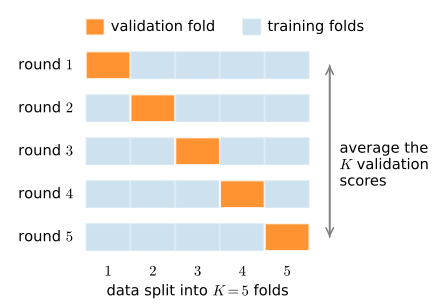
How should we choose \(K\)? The choice trades off bias, variance, and compute. Each fold’s model is trained on only \((K-1)/K\) of the data. If the learning curve improves monotonically with sample size, its error is higher than that of the model finally trained on all the data, making the cross-validation estimate pessimistic. This conclusion is not guaranteed for unstable or non-monotone learning procedures. Taking \(K = n\) (leave-one-out cross-validation) all but eliminates this bias, but at a steep price: it requires \(n\) model fits, and the \(n\) training sets are nearly identical, so the fold errors are highly correlated and their average tends to have higher variance; in fact no general unbiased estimator of the cross-validation variance exists (Bengio and Grandvalet 2004). The standard compromise, \(K = 5\) or \(K = 10\), keeps the bias modest, averages over reasonably distinct training sets, and costs only \(5\)–\(10\) fits, which is why these values dominate practice (Kohavi 1995). (Exercises 4 and 5 ask you to reason through the cost and the bias.)
2.6.4 Summary
Generalization concerns the difference between performance on the training sample and performance on new data from the same distribution. The following principles guide model selection in the settings considered here:
- Use validation sets (or \(K\)-fold cross-validation) for model selection;
- More complex models often require more data;
- Relevant notions of complexity include both the number of parameters and the range of values that they are allowed to take;
- Keeping the learning procedure and data distribution fixed, more data usually improves generalization, but the curve need not be monotone;
- These conclusions assume that training and test data are IID. Distribution shift requires additional assumptions.
2.6.5 Exercises
Exact polynomial regression. State the condition under which polynomial regression can be solved exactly. Hint: relate the polynomial degree to the number of distinct data points.
When IID fails. Give at least five examples where dependent random variables make treating the problem as IID data inadvisable.
Two kinds of zero training error. State whether zero training error is achievable in practice. Under which circumstances would zero generalization error be achievable? Distinguish the two cases clearly.
The price of \(K\)-fold. Explain why \(K\)-fold cross-validation is very expensive to compute, in terms of the number of models fit relative to a single train/validation split.
\(K\)-fold bias. Explain why the \(K\)-fold cross-validation error estimate is biased relative to a model trained on the full dataset, and state the direction of the bias.
VC dimension. It is defined as the maximum number of points that can be classified with arbitrary labels \(\{\pm 1\}\) by a function of a class of functions. Why might this not be a good idea for measuring how complex the class of functions is? Hint: consider the magnitude of the function values, rather than just the signs.
[code] Learning curve. Your manager gives you a difficult dataset on which your current algorithm does not perform so well, and you cannot collect more data. Subsample the existing training set at several sizes, for example 20%, 40%, 60%, 80%, and 100%, retrain at each size, and plot validation error against training-set size. How would you use the slope of the resulting curve as evidence whether more data might help?
[code] Model selection. Re-run the polynomial-fitting experiment above with
n_trainset to 10, 40, and 100. Report the degree at which the test loss starts to climb in each case, and relate your finding to the rule of thumb that more complex models require more data.[extended] Double Descent. ● Extend this section’s polynomial-degree sweep well past the number of training points, for example to degree 60 on 20 training points, relying on the minimum-norm behavior of
lstsqin the rank-deficient regime. Before running it, predict whether the test error keeps rising once the training error reaches zero, or falls again. Then run the sweep, plot the test error across the full range, and relate the outcome to this section’s discussion of double descent.Adapted from Simon Prince, Understanding Deep Learning, Problem 8.4.