%matplotlib inline
import math
import numpy as onp
from d2l import torch as d2l
import torch25.1 Single Variable Calculus
This section develops the one-variable calculus used in deep learning. The derivative provides a local linear approximation, and a small set of rules computes derivatives of composite expressions. We use this approximation to derive gradient descent, introduce curvature and Taylor series, and examine nondifferentiable points such as the corner of \(\mathrm{ReLU}\).
25.1.1 The Derivative
Differential calculus describes how a function responds to a small change in its input. Let \(L(\mathbf w)\) denote the training loss of a neural network whose weights are collected in \(\mathbf w=(w_1,\ldots,w_n)\). Direct minimization is generally unavailable, so training repeatedly updates the parameters against the gradient,
\[ \mathbf{w} \leftarrow \mathbf{w} - \eta\, \nabla L(\mathbf{w}), \]
where \(\nabla L(\mathbf{w})\) (defined in Section 25.2) collects the derivatives with respect to all weights, and \(\eta>0\) is the step size. We first hold all but one weight fixed and study the one-variable slice \(f(x)=L(w_1,\ldots,x,\ldots,w_n)\).
25.1.1.1 Local Linear Approximation
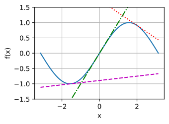
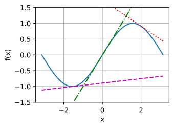
Consider a point \(x\) and a small perturbation \(\epsilon\). A nonlinear function, such as the smooth curve in Figure 25.1.1, becomes increasingly close to its tangent line on smaller neighborhoods of a differentiable point. Figure 25.1.1 shows three successively smaller windows.
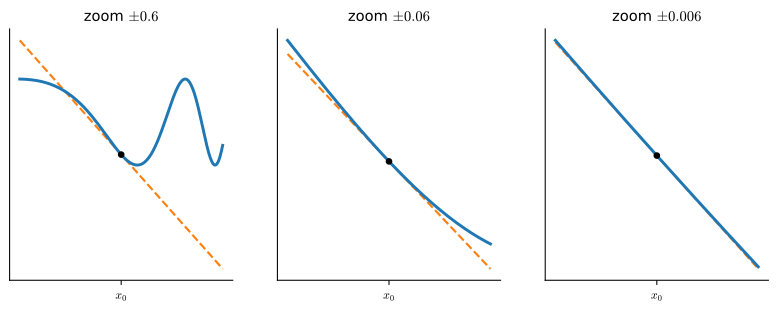
At a differentiable point, the tangent is a first-order approximation: after a step \(\epsilon\), the approximation error is negligible relative to \(|\epsilon|\) as \(\epsilon\to0\). The proportionality between the leading input and output changes is the tangent slope.
25.1.1.2 The Difference Quotient and the Derivative
To measure that slope we compare the change in output to the change in input,
\[ \frac{f(x+\epsilon) - f(x)}{(x+\epsilon) - x} = \frac{f(x+\epsilon) - f(x)}{\epsilon}, \]
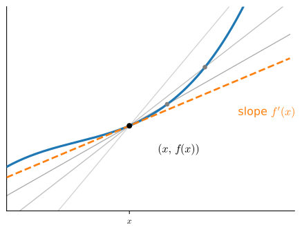
the slope of the secant line through \((x, f(x))\) and \((x+\epsilon, f(x+\epsilon))\). As \(\epsilon\) shrinks, the second point approaches the first and the secant slope approaches the tangent slope, as shown in Figure 25.1.2. The following computation measures this convergence. We use these imports throughout the section.
%matplotlib inline
import math
import numpy as onp
from d2l import tensorflow as d2l
import tensorflow as tf%matplotlib inline
import math
import numpy as onp
from d2l import jax as d2l
import jax
from jax import numpy as jnp%matplotlib inline
import math
import numpy as onp
from d2l import mxnet as d2l
from mxnet import autograd, np, npx
npx.set_np()Take \(f(x) = x^2 + 1701(x-4)^3\) and evaluate the difference quotient at \(x = 4\) for shrinking \(\epsilon\).
# Define our function
def f(x):
    return x**2 + 1701*(x-4)**3

# Slope of the secant through x=4, for shrinking epsilon
for epsilon in [0.1, 0.001, 0.0001, 0.00001]:
    print(f'epsilon = {epsilon:.5f} -> {(f(4+epsilon) - f(4)) / epsilon:.5f}')
epsilon = 0.10000 -> 25.11000
epsilon = 0.00100 -> 8.00270
epsilon = 0.00010 -> 8.00012
epsilon = 0.00001 -> 8.00001The values converge to \(8\) as \(\epsilon\) decreases. Expanding \(f(4+\epsilon)-f(4)=8\epsilon+\epsilon^2+1701\epsilon^3\) gives the difference quotient \(8+\epsilon+1701\epsilon^2\). The cubic contributes an error of \(17\) at \(\epsilon=0.1\) but only \(1.7\times10^{-7}\) at \(\epsilon=10^{-5}\). Thus the slope at \(x=4\) is \(8\), written
\[ \lim_{\epsilon \rightarrow 0}\frac{f(4+\epsilon) - f(4)}{\epsilon} = 8. \]
The table approaches the limit through finite differences. Automatic differentiation (Section 1.5) instead applies exact differentiation rules in floating-point arithmetic, so it introduces no \(\epsilon\) or truncation error; only rounding remains. For the same \(f\) at \(x = 4\), it returns \(8\). The rules below formalize this calculation, and Section 25.3 builds an automatic differentiation system from them.
# Autograd computes the limit exactly: f'(4) = 8
x = torch.tensor(4.0, requires_grad=True)
f(x).backward()
print(f"autograd: f'(4) = {x.grad.item():.1f}")
autograd: f'(4) = 8.0# Autograd computes the limit exactly: f'(4) = 8
x = tf.Variable(4.0)
with tf.GradientTape() as t:
y = f(x)
print(f"autograd: f'(4) = {t.gradient(y, x).numpy():.1f}")autograd: f'(4) = 8.0# Autograd computes the limit exactly: f'(4) = 8
print(f"autograd: f'(4) = {jax.grad(f)(4.0):.1f}")autograd: f'(4) = 8.0# Autograd computes the limit exactly: f'(4) = 8
x = np.array(4.0)
x.attach_grad()
with autograd.record():
y = f(x)
y.backward()
print(f"autograd: f'(4) = {float(x.grad):.1f}")autograd: f'(4) = 8.0[21:23:57] /home/smola/mxnet/src/base.cc:48: GPU context requested, but no GPUs found.This computation is the method of finite differences. It measures a weight’s effect on the loss by perturbing that weight and evaluating the network again. It costs an extra evaluation of \(L\) per weight (or two, for the centered differences that halve the truncation error), so with even a few thousand parameters it is thousands of forward passes for a single gradient. The backpropagation algorithm popularized in 1986 by Rumelhart et al. (1986) removes that bottleneck: it delivers the effect of all weights at once, at a small constant multiple of the cost of one forward pass, the cheap-gradient principle (Griewank and Walther 2008). Backpropagation is the chain rule (below) run in reverse over the network.
The slope is itself a function of \(x\), so we name it. The derivative of \(f\) is
\[\frac{df}{dx}(x) = \lim_{\epsilon \rightarrow 0}\frac{f(x+\epsilon) - f(x)}{\epsilon}, \tag{25.1.1}\]
when the limit exists. (When it fails to, as at the corner of \(\mathrm{ReLU}\), we will need the refinement of Section 25.1.5.) Many notations denote this same object, and all of them appear in the literature:
\[ \frac{df}{dx} = \frac{d}{dx}f = f' = D_xf = f_x. \]
We default to \(\frac{df}{dx}\), switching to \(\frac{d}{dx}f\) when differentiating a bulky expression such as \(\frac{d}{dx}\left[x^4+\cos\left(\frac{x^2+1}{2x-1}\right)\right]\).
25.1.1.3 The Small-Change Identity
Rearranging the definition gives an identity that turns knowledge of the derivative into a prediction of the function’s values nearby. Since the quotient approaches the derivative, for small \(\epsilon\)
\[ \frac{f(x+\epsilon) - f(x)}{\epsilon} \approx \frac{df}{dx}(x) \quad\Longrightarrow\quad f(x+\epsilon) \approx f(x) + \epsilon \frac{df}{dx}(x). \tag{25.1.2}\]
Thus a perturbation \(\epsilon\) changes the output by \(\epsilon f'(x)\) to first order. We use “\(\approx\)” to omit terms that vanish faster than \(\epsilon\) as \(\epsilon\to0\). Formally, if \(o(\epsilon)/\epsilon\to0\), then Equation 25.1.2 reads \(f(x+\epsilon)=f(x)+\epsilon f'(x)+o(\epsilon)\). This local approximation will be used to derive differentiation rules, gradient descent, and Taylor series.
25.1.2 Computing Derivatives
Rather than deriving every elementary derivative from the limit Equation 25.1.1, we use a short table of derivatives for the elementary functions, plus a handful of rules for combining them, from which any expression built out of sums, products, quotients, and compositions can be differentiated mechanically.
25.1.2.1 A Table of Common Derivatives
As in Section 1.4, most derivatives reduce to a few core ones, repeated here for reference.
- Derivative of constants. \(\frac{d}{dx}c = 0\).
- Derivative of linear functions. \(\frac{d}{dx}(ax) = a\).
- Power rule. \(\frac{d}{dx}x^n = nx^{n-1}\).
- Derivative of exponentials. \(\frac{d}{dx}e^x = e^x\).
- Derivative of the logarithm. \(\frac{d}{dx}\log(x) = \frac{1}{x}\).
- Derivative of sine. \(\frac{d}{dx}\sin(x) = \cos(x)\).
- Derivative of cosine. \(\frac{d}{dx}\cos(x) = -\sin(x)\).
(That \(e^x\) is its own derivative is the small-change identity in disguise: \(e^{x+\epsilon} = e^x e^{\epsilon} \approx e^x(1 + \epsilon)\), so the coefficient of \(\epsilon\) is \(e^x\) itself. This takes the first-order expansion \(e^{\epsilon} \approx 1 + \epsilon\) as given, since that expansion is the table entry at \(x = 0\); the aside is intuition for the entry, not an independent proof of it.)
25.1.2.2 Rules for Combining Derivatives
Derivatives respect addition, multiplication, division, and composition. Therefore, the following rules differentiate any expression assembled from the table:
- Sum rule. \(\frac{d}{dx}\left(g(x) + h(x)\right) = \frac{dg}{dx}(x) + \frac{dh}{dx}(x)\).
- Product rule. \(\frac{d}{dx}\left(g(x)\, h(x)\right) = g(x)\frac{dh}{dx}(x) + \frac{dg}{dx}(x)h(x)\).
- Quotient rule. \(\frac{d}{dx}\left(\frac{g(x)}{h(x)}\right) = \frac{\frac{dg}{dx}(x)h(x) - g(x)\frac{dh}{dx}(x)}{h(x)^2}\), valid wherever \(h(x)\neq 0\).
- Chain rule. \(\frac{d}{dx}g(h(x)) = \frac{dg}{dh}(h(x))\cdot \frac{dh}{dx}(x)\).
Each rule follows by writing \(f(x+\epsilon)\), expanding its factors to first order, and collecting the coefficient of \(\epsilon\) according to Equation 25.1.2.
Sum rule. Expanding each summand,
\[ f(x+\epsilon) = g(x+\epsilon) + h(x+\epsilon) \approx \Bigl(g(x) + h(x)\Bigr) + \epsilon\left(\frac{dg}{dx}(x) + \frac{dh}{dx}(x)\right), \]
so the coefficient of \(\epsilon\), the derivative, is \(\frac{dg}{dx}(x) + \frac{dh}{dx}(x)\). The two first-order changes add. \(\blacksquare\)
Product rule. Expanding both factors and multiplying out,
\[ \begin{aligned} f(x+\epsilon) = g(x+\epsilon)\,h(x+\epsilon) &\approx \left(g(x) + \epsilon g'(x)\right)\left(h(x) + \epsilon h'(x)\right) \\ &= g(x)h(x) + \epsilon\Bigl(g(x)h'(x) + g'(x)h(x)\Bigr) + \underbrace{\epsilon^2\, g'(x)h'(x)}_{\textrm{higher order}}. \end{aligned} \]
The \(\epsilon^2\) term is a higher-order term: with \(\epsilon = 10^{-7}\) it is \(10^{-14}\), dwarfed by the \(\epsilon\) term, and it vanishes faster than \(\epsilon\) as \(\epsilon \to 0\). Dropping it, the coefficient of \(\epsilon\) gives \(g(x)h'(x) + g'(x)h(x)\). The lopsided shape, differentiate one factor, leave the other alone, then swap, is exactly the two ways a rectangle of sides \(g\) and \(h\) grows when both sides stretch. (If you want to avoid “\(\approx\)” entirely, divide the line above by \(\epsilon\): the difference quotient equals \(g(x)h'(x)+g'(x)h(x) + \epsilon\,g'(x)h'(x)\), whose last term goes to \(0\).) \(\blacksquare\)
Chain rule. Compose, then expand the inner function first and feed the result into the outer one:
\[ \begin{aligned} f(x+\epsilon) &= g\bigl(h(x+\epsilon)\bigr)\\ &\approx g\!\left(h(x) + \epsilon\, h'(x)\right) &&\text{(inner: small-change identity)}\\ &\approx g(h(x)) + \epsilon\, h'(x)\, \frac{dg}{dh}(h(x)) &&\text{(outer: small-change identity, with step } \epsilon h'(x)). \end{aligned} \]
The coefficient of \(\epsilon\) is \(\frac{dg}{dh}(h(x))\, h'(x)\): a change in \(x\) moves \(h\) by \(\epsilon h'(x)\), and that in turn moves \(g\) by its own derivative times that step: the rates multiply. The one subtlety is the second line, where we fed the variable step \(\epsilon h'(x)\) into \(g\)’s small-change identity: because \(g\) is differentiable at \(h(x)\), its error term is \(o(\text{step}) = o(\epsilon h'(x))\) in the \(o(\cdot)\) notation we fixed after Equation 25.1.2, which is still \(o(\epsilon)\) and so vanishes faster than the \(\epsilon\) we keep. (The borderline case \(h'(x) = 0\), where the step degenerates, is handled by the standard error-function form of the proof: write \(g(h(x)+s) = g(h(x)) + (g'(h(x)) + r(s))\,s\) with \(r(s)\to 0\), substitute \(s = \epsilon h'(x) + o(\epsilon)\), and the same coefficient drops out.) Applied across the layers of a network, this chaining of local linear factors is the backpropagation we met above. (The quotient rule is the product and chain rules applied to \(g\cdot h^{-1}\); we leave it as Exercise 2.) \(\blacksquare\)
The chain rule also gives the derivative of an inverse function. If \(g\) undoes \(f\), meaning \(g(f(x)) = x\), then differentiating both sides gives \(g'(f(x))\,f'(x) = 1\), so \(g'(y) = 1/f'(g(y))\) wherever \(f'(g(y)) \neq 0\): the slope of the inverse is the reciprocal slope, read at the matching point (the graph of \(g\) is the graph of \(f\) flipped across the diagonal, which turns rise-over-run upside down). This is where the logarithm’s entry in the table comes from: \(\log\) undoes \(e^x\), so \(\frac{d}{dx}\log(x) = 1/e^{\log x} = 1/x\). The deep-learning instance is the sigmoid \(\sigma(x) = 1/(1+e^{-x})\), with \(\sigma' = \sigma(1-\sigma)\), and its inverse the logit \(\log\frac{p}{1-p}\), whose derivative \(\frac{1}{p(1-p)}\) is exactly the reciprocal of \(\sigma'\) evaluated at the matching point.
Together these rules let us differentiate essentially anything in closed form. For instance,
\[ \begin{aligned} \frac{d}{dx}\left[\log\left(1+(x-1)^{10}\right)\right] & = \left(1+(x-1)^{10}\right)^{-1}\frac{d}{dx}\left[1+(x-1)^{10}\right]\\ & = \left(1+(x-1)^{10}\right)^{-1}\left(\frac{d}{dx}[1] + \frac{d}{dx}[(x-1)^{10}]\right) \\ & = \left(1+(x-1)^{10}\right)^{-1}\left(0 + 10(x-1)^9\frac{d}{dx}[x-1]\right) \\ & = 10\left(1+(x-1)^{10}\right)^{-1}(x-1)^9 \\ & = \frac{10(x-1)^9}{1+(x-1)^{10}}. \end{aligned} \]
Where each line has used the following rules:
- The chain rule and derivative of logarithm.
- The sum rule.
- The derivative of constants, chain rule, and power rule.
- The sum rule, derivative of linear functions, derivative of constants.
Two lessons follow. First, anything assembled from sums, products, constants, powers, exponentials, and logarithms can be differentiated mechanically. Second, doing so by hand is tedious and error-prone, which is exactly why automatic differentiation (Section 1.5) mechanizes it.
25.1.3 Linear Approximation and Gradient Descent
The small-change identity is the bridge from computing derivatives to using them for optimization. We first read it geometrically as the tangent line, then turn it into the gradient-descent step.
25.1.3.1 The Tangent Line
Reading Equation 25.1.2 as a function of the displacement, the line
\[ f(x+\epsilon) \approx f(x) + \epsilon \frac{df}{dx}(x) \]
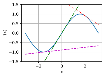
passes through \((x, f(x))\) with slope \(\frac{df}{dx}(x)\): it is the tangent at \(x\), the best straight-line model of \(f\) nearby and the limit of the rotating secants of Figure 25.1.2. Drawing the tangent at several points of \(\sin\), using \(\frac{d}{dx}\sin(x) = \cos(x)\), shows that each line approximates the curve well near its base point and diverges from it farther away.
import numpy as onp
# Compute sin
xs = onp.arange(-onp.pi, onp.pi, 0.01)
plots = [onp.sin(xs)]

# Compute some linear approximations. Use d(sin(x)) / dx = cos(x)
for x0 in [-1.5, 0, 2]:
    plots.append(onp.sin(x0) + (xs - x0) * onp.cos(x0))

d2l.plot(xs, plots, 'x', 'f(x)', ylim=[-1.5, 1.5])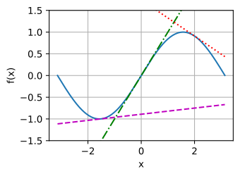
25.1.3.2 The Gradient-Descent Step
The step \(\epsilon\) can also be chosen to reduce the function value. In the small-change identity Equation 25.1.2 the step \(\epsilon\) is ours to pick, and we want to pick it so that \(f\) goes down. The identity already predicts the effect of any step: a step \(\epsilon\) changes the output by about \(\epsilon\, f'(x)\). To make that change negative, point the step opposite the slope: take \(\epsilon = -\eta\, f'(x)\) for a step size \(\eta > 0\), and, if the step is not too large, the descent is guaranteed.
The qualification matters. The small-change identity by itself only describes the first-order model; turning “the model goes down” into “\(f\) really goes down” needs control on how fast the slope can change over the step, which is exactly the curvature. The standard hypothesis is that \(f'\) is \(L\)-Lipschitz near \(x\), meaning \(|f'(u) - f'(v)| \le L\,|u-v|\) for \(u,v\) in a neighborhood, so the slope cannot swing by more than \(L\) per unit of \(x\). (If \(f\) is twice differentiable this just says \(|f''| \le L\) there.) Under that single assumption the first-order guess becomes a genuine inequality, the descent lemma of smooth optimization (Nesterov 2018).
Proposition (descent lemma). Suppose \(f'\) is \(L\)-Lipschitz on a neighborhood of \(x\). Then for every step size \(\eta > 0\) small enough that the segment stays in that neighborhood,
\[ f\bigl(x - \eta\, f'(x)\bigr) \;\le\; f(x) - \eta\left(1 - \tfrac{L\eta}{2}\right)[f'(x)]^2. \tag{25.1.3}\]
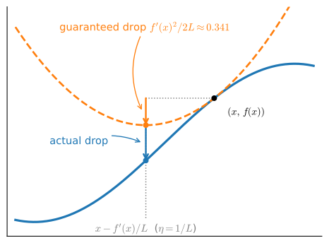
In particular \(f\) strictly decreases whenever \(0 < \eta < 2/L\) and \(f'(x) \neq 0\), and the guaranteed decrease is largest at the step \(\eta = 1/L\), where the bound reads \(f(x - \tfrac1L f'(x)) \le f(x) - \tfrac{1}{2L}[f'(x)]^2\).
Proof. Write the exact change in \(f\) along the step as an integral of the slope, using the fundamental theorem of calculus (which we take on faith until Section 25.4), then add and subtract the slope at the base point:
\[ f(x+s) - f(x) = \int_0^1 f'(x + t s)\, s \, dt = f'(x)\, s + \int_0^1 \bigl(f'(x + t s) - f'(x)\bigr) s\, dt. \]
Bounding the remaining integrand with the Lipschitz hypothesis, \(|f'(x+ts) - f'(x)| \le L\,|ts| = Lt|s|\), and using \(\int_0^1 t\, dt = \tfrac12\) gives \(f(x+s) \le f(x) + f'(x)\,s + \tfrac{L}{2}s^2\). Now insert the descent step \(s = -\eta\,f'(x)\):
\[ f\bigl(x - \eta\, f'(x)\bigr) \le f(x) - \eta\,[f'(x)]^2 + \tfrac{L}{2}\eta^2 [f'(x)]^2 = f(x) - \eta\left(1 - \tfrac{L\eta}{2}\right)[f'(x)]^2. \]
The bracket \(1 - L\eta/2\) is positive exactly for \(\eta < 2/L\), and as a function of \(\eta\) the whole coefficient \(\eta(1 - L\eta/2)\) is maximized at \(\eta = 1/L\). \(\blacksquare\)
Figure 25.1.3 illustrates the bound \(f(x+s)\le f(x)+f'(x)s+\tfrac{L}{2}s^2\). The quadratic upper bound touches the function at the base point. Its minimizer is the gradient step with \(\eta=1/L\), where the bound has decreased by \(\tfrac{1}{2L}[f'(x)]^2\). The actual decrease can be larger.
The first-order decrease is \(-\eta[f'(x)]^2\), while curvature contributes the second-order term \(\tfrac{L}{2}\eta^2[f'(x)]^2\). The former dominates when \(\eta<2/L\). Consequently, moving against a nonzero slope decreases \(f\) by an amount controlled by the squared slope. Iterating this update gives one-dimensional gradient descent,
\[ x_{t+1} = x_t - \eta\, f'(x_t), \tag{25.1.4}\]
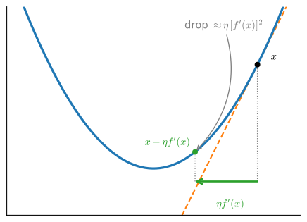
which is exactly the weight update \(\mathbf{w} \leftarrow \mathbf{w} - \eta\,\nabla L(\mathbf{w})\) from the introduction, one coordinate at a time. Figure 25.1.4 shows how a step of \(-\eta f'(x)\) from \(x\) moves in the direction opposite the slope and decreases the local linear model.
Two consequences follow. At the stationary condition \(f'(x)=0\), the update stops and Equation 25.1.3 predicts no further decrease, so stationary points are candidates for minima. The guaranteed decrease holds only for \(\eta<2/L\); at \(\eta=2/L\), the second-order contribution cancels the first-order decrease. For larger steps, a single update can overshoot a minimum and increase \(f\), as analyzed in Section 9.2. Thus the Lipschitz constant \(L\) determines the range of step sizes covered by the guarantee and measures the curvature considered next.
We can see all of this on the simplest example, \(f(x) = x^2\), whose slope is \(f'(x) = 2x\). The gradient-descent step becomes
\[ x_{t+1} = x_t - \eta\,(2x_t) = (1 - 2\eta)\, x_t, \]
a simple geometric recursion with closed form \(x_t = (1-2\eta)^t x_0\). So the iterates converge to the minimum \(x = 0\) exactly when \(|1 - 2\eta| < 1\), i.e. for \(0 < \eta < 1\). This is the descent lemma made exact: here \(f'' \equiv 2\) so \(L = 2\) and the safe range \(\eta < 2/L = 1\) is precisely the convergence threshold. Within it, a small \(\eta\) converges monotonically but slowly, the optimal \(\eta = 1/L = \tfrac12\) reaches the minimum in one step, \(\tfrac12 < \eta < 1\) overshoots and oscillates inward, \(\eta = 1\) oscillates forever between \(\pm x_0\), and \(\eta > 1\) diverges. The next code cell runs the recursion for a sweep of step sizes, prints the value of each iterate after ten steps, and plots the five trajectories \(x_t\).
# Gradient descent on f(x) = x^2 from x0 = 1, for several step sizes
def gd(eta, steps=10, x0=1.0):
    xs = [x0]
    for _ in range(steps):
        xs.append(xs[-1] - eta * (2 * xs[-1]))  # x <- x - eta * f'(x)
    return xs

etas = [0.05, 0.5, 0.9, 1.0, 1.1]
trajectories = [gd(eta) for eta in etas]
for eta, xs in zip(etas, trajectories):
    print(f'eta = {eta:.2f} -> x_10 = {xs[-1]:+.5f}')
d2l.plot(list(range(11)), trajectories, 'step t', 'x_t', ylim=[-2.5, 2.5],
         legend=[f'eta = {eta}' for eta in etas],
fmts=('-', 'm--', 'g-.', 'r:', 'c-'))eta = 0.05 -> x_10 = +0.34868
eta = 0.50 -> x_10 = +0.00000
eta = 0.90 -> x_10 = +0.10737
eta = 1.00 -> x_10 = +1.00000
eta = 1.10 -> x_10 = +6.19174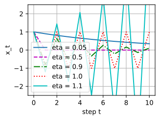
eta = 0.05 -> x_10 = +0.34868
eta = 0.50 -> x_10 = +0.00000
eta = 0.90 -> x_10 = +0.10737
eta = 1.00 -> x_10 = +1.00000
eta = 1.10 -> x_10 = +6.19174
eta = 0.05 -> x_10 = +0.34868
eta = 0.50 -> x_10 = +0.00000
eta = 0.90 -> x_10 = +0.10737
eta = 1.00 -> x_10 = +1.00000
eta = 1.10 -> x_10 = +6.19174
eta = 0.05 -> x_10 = +0.34868
eta = 0.50 -> x_10 = +0.00000
eta = 0.90 -> x_10 = +0.10737
eta = 1.00 -> x_10 = +1.00000
eta = 1.10 -> x_10 = +6.19174
The printout and figure show one regime per curve: \(\eta = 0.05\) converges slowly and monotonically to \(0\), \(\eta = 0.5\) reaches it in a single step, \(\eta = 0.9\) converges while alternating across the minimum, \(\eta = 1.0\) alternates between \(\pm 1\) indefinitely, and \(\eta = 1.1\) oscillates with growing amplitude: it has left the plotting window within a handful of steps and reaches \(|x_{10}| \approx 6.2\). The threshold \(\eta = 2/L\) separating the last two regimes is exactly where the descent lemma’s guarantee expires.
25.1.4 Curvature and Taylor Series
The first derivative gave us the best line through a point. Its own derivative, the second derivative, measures how the slope itself bends, which is what distinguishes a minimum from a maximum and what limited the step size above. Pushing the idea to higher derivatives yields the Taylor series, the best polynomial model of a function.
25.1.4.1 Higher-Order Derivatives and Curvature
The derivative \(\frac{df}{dx}\) is itself a function, so nothing stops us from differentiating it again. Doing so yields the second derivative, \(\frac{d^2f}{dx^2} = \frac{d}{dx}\!\left(\frac{df}{dx}\right)\): the derivative operator applied twice, not the square of \(\frac{df}{dx}\). It is the rate of change of the rate of change: how the slope itself is changing. Repeating gives the \(n\)-th derivative,
\[ f^{(n)}(x) = \frac{d^{n}f}{dx^{n}} = \left(\frac{d}{dx}\right)^{n} f. \]
What does the second derivative tell us? Its sign is the direction the curve bends, and read locally this is the classifier we need for optimization. Suppose \(x_0\) is a stationary point, \(f'(x_0) = 0\). Then the definition of the second derivative collapses to \(f''(x_0) = \lim_{h \to 0} f'(x_0+h)/h\); if that limit is positive, the quotient \(f'(x_0+h)/h\) is positive for all small \(h \neq 0\), so \(f'(x_0+h)\) shares the sign of \(h\): just left of \(x_0\) the slope is negative (\(f\) falling), just right of \(x_0\) it is positive (\(f\) rising). The function dips and turns back up, so \(x_0\) is a local minimum. Symmetrically, \(f''(x_0) < 0\) makes the slope positive then negative, so \(f\) rises and turns back down and \(x_0\) is a local maximum. This is the second-derivative test, and it certifies only the neighborhood of \(x_0\), not the whole function; for the global picture, when \(f\) is convex, see Section 9.2.
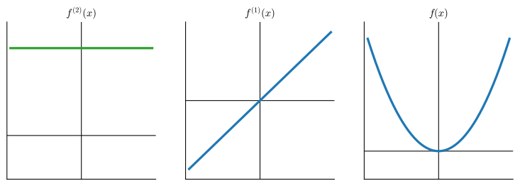
The three constant-curvature functions show what each sign means, even though most functions have a varying \(f''\). A positive constant \(f''\) keeps the slope increasing everywhere, so \(f'\) runs from negative through zero to positive and the graph is a single upward bowl (Figure 25.1.5), exactly the bowl that gradient descent rolls into.
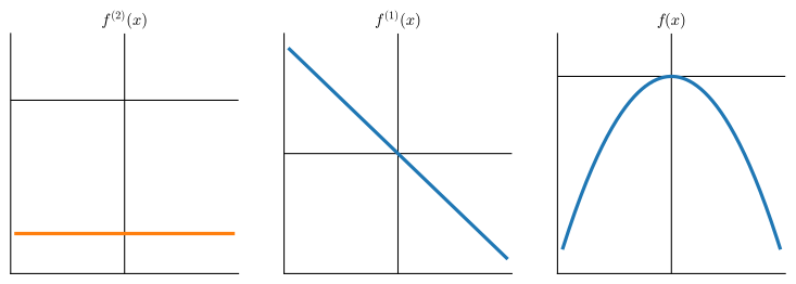
A negative constant \(f''\) keeps the slope decreasing, running from positive through zero to negative: the upward dome of a maximum (Figure 25.1.6).
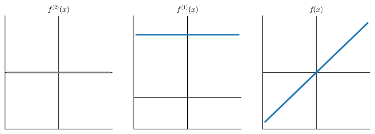
And a zero \(f''\) leaves the slope unchanged: \(f\) rises or falls at a fixed rate and is a straight line with no curvature at all (Figure 25.1.7), the borderline the test cannot decide.
In short, the sign of the second derivative at a stationary point decides minimum versus maximum: positive curves up into a min, negative curves down into a max, zero is undecided. (This is the one-dimensional shadow of the Hessian eigenvalue test for many variables in Section 25.2.)
25.1.4.2 The Mean Value Theorem
We have been spending the derivative freely: a vanishing slope marks a candidate extremum, a negative slope means the function is falling. Both deductions read information about \(f\) itself off its derivative at single points, and one theorem licenses every such reading: the Mean Value Theorem. Its statement is a picture (Figure 25.1.8): draw the secant chord joining the endpoints of the graph over \([a,b]\); somewhere inside, the tangent runs parallel to it. The average rate of change is achieved exactly, as an instantaneous rate, at some interior point.
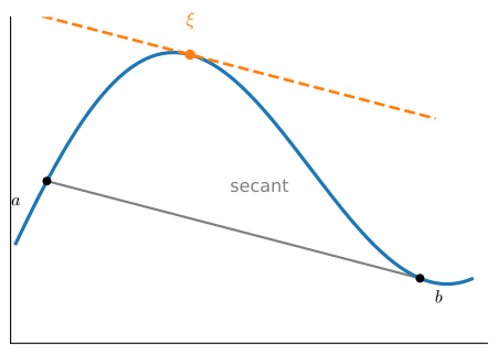
Proposition (Mean Value Theorem). If \(f\) is continuous on \([a,b]\) and differentiable on \((a,b)\), then there is a point \(\xi \in (a,b)\) with
\[ f'(\xi) = \frac{f(b) - f(a)}{b - a}. \tag{25.1.5}\]
Proof. First take the flat case \(f(a) = f(b)\) (Rolle’s theorem). We grant ourselves one fact from real analysis, the extreme value theorem: a continuous function on a closed interval attains a maximum and a minimum (Rudin 1976). If both occur at the endpoints then \(f\) is constant and \(f' \equiv 0\) inside; otherwise an extremum sits at some interior \(\xi\), say a maximum, so \(f(\xi + \epsilon) - f(\xi) \le 0\) on both sides. The difference quotient is then \(\le 0\) for \(\epsilon > 0\) and \(\ge 0\) for \(\epsilon < 0\), and since \(f\) is differentiable at \(\xi\) both one-sided limits equal \(f'(\xi)\); a number that is both \(\le 0\) and \(\ge 0\) is zero, so \(f'(\xi) = 0\) (a minimum is symmetric). For the general case, subtract off the chord: the tilted function \(g(x) = f(x) - \frac{f(b)-f(a)}{b-a}(x - a)\) has \(g(a) = g(b) = f(a)\), so the flat case gives a \(\xi\) with \(g'(\xi) = 0\), which is exactly Equation 25.1.5. \(\blacksquare\)
Two corollaries are the facts we already used. If \(f' > 0\) throughout an interval then for any \(x_1 < x_2\) in it, Equation 25.1.5 gives \(f(x_2) - f(x_1) = f'(\xi)(x_2 - x_1) > 0\) for some \(\xi\) between them, so \(f\) is increasing: a positive slope really does mean the function climbs, and the sign of \(f'\) governs monotonicity. And if \(f\) has a constant sign of \(f'\) on each side of a stationary point, the theorem turns that into the rise-and-fall behaviour the second-derivative test read off. The Mean Value Theorem is the formal bridge from the derivative at a point to the behaviour of the function on an interval.
25.1.4.3 Quadratic Approximation and the Taylor Expansion
The first derivative built the best line; the second lets us build the best parabola. Consider a generic quadratic \(g(x) = ax^2 + bx + c\), for which
\[ \begin{aligned} \frac{dg}{dx}(x) & = 2ax + b \\ \frac{d^2g}{dx^2}(x) & = 2a. \end{aligned} \]
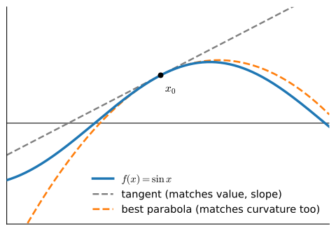
A quadratic has three free coefficients, so we can match three pieces of information about \(f\) at a base point \(x_0\): its value, slope, and curvature. Demanding \(g(x_0) = f(x_0)\), \(g'(x_0) = f'(x_0)\), and \(g''(x_0) = f''(x_0)\) pins down \(a\), \(b\), \(c\) uniquely and produces the best local quadratic model, just as the tangent was the best local line. For \(f(x) = \sin(x)\) at base point \(x_0\), using \(\frac{d}{dx}\sin(x) = \cos(x)\) and \(\frac{d^2}{dx^2}\sin(x) = -\sin(x)\), the model reads
\[ g(x) = \sin(x_0) + \cos(x_0)\,(x - x_0) - \tfrac{1}{2}\sin(x_0)\,(x-x_0)^2, \]
a parabola that remains accurate over a visibly wider interval than the tangent lines plotted above because it captures curvature as well as slope; Figure 25.1.9 draws all three together. We will make the “wider window” claim quantitative, and verify it in code, once the Taylor remainder is on the table. But first, the quadratic model changes how we optimize.
25.1.4.4 Newton’s Method
The quadratic model supplies a candidate step rather than an automatic improvement. When \(f''(x_t)>0\), its local model opens upward and has a unique minimizer. Writing that model at the current iterate,
\[ q(x) = f(x_t) + f'(x_t)\,(x - x_t) + \tfrac{1}{2}f''(x_t)\,(x - x_t)^2, \]
and solving \(q'(x) = f'(x_t) + f''(x_t)(x - x_t) = 0\) for \(x\) gives the update of Newton’s method:
\[ x_{t+1} = x_t - \frac{f'(x_t)}{f''(x_t)}. \tag{25.1.6}\]
For positive curvature, this resembles a gradient step with the local scale \(1/f''(x_t)\). On \(f(x)=x^2\) it reaches the minimizer in one step. More generally, if \(f''\) is Lipschitz near a local minimizer \(x^\star\), \(f''(x^\star)>0\), and the iteration begins sufficiently close, Newton’s method converges quadratically (Nocedal and Wright 2006). Outside that local regime a full step may increase the true objective; if curvature is nonpositive or nearly zero, the quadratic minimizer is absent or unstable. Damping and trust-region methods safeguard the step. In \(n\) dimensions the curvature becomes a Hessian, and each Newton step requires solving a linear system; Section 26.1 develops this tradeoff.
The quadratic convergence is easy to watch. Take \(f(x) = \tfrac14 x^4 - x\), whose stationarity condition \(f'(x) = x^3 - 1 = 0\) has the root \(x^* = 1\); the next cell iterates Equation 25.1.6 from \(x_0 = 2\) and prints the error at each step.
# Newton's method on f(x) = x^4/4 - x: solve f'(x) = x^3 - 1 = 0, root x* = 1
x = 2.0
for t in range(6):
    print(f't = {t}: x = {x:.12f}, error = {abs(x - 1):.1e}')
    x = x - (x**3 - 1) / (3 * x**2)  # x - f'(x) / f''(x)
t = 0: x = 2.000000000000, error = 1.0e+00
t = 1: x = 1.416666666667, error = 4.2e-01
t = 2: x = 1.110534409842, error = 1.1e-01
t = 3: x = 1.010636768405, error = 1.1e-02
t = 4: x = 1.000111557304, error = 1.1e-04
t = 5: x = 1.000000012443, error = 1.2e-08After the first few steps, the error exponents progress as \(10^{-2} \to 10^{-4} \to 10^{-8}\): each step roughly squares the previous error, doubling the number of correct digits. Contrast the \(\eta\)-sweep above, where gradient descent shrinks the error by the same fixed factor \(|1 - 2\eta|\) every step: geometric convergence gains a fixed number of digits per step, Newton doubles them. Matching yet more derivatives with higher-degree polynomials is the Taylor series, to which we now turn.
25.1.4.5 Taylor Series
The Taylor series generalizes the tangent and the best parabola: given the value and first \(n\) derivatives of \(f\) at a base point \(x_0\), find the degree-\(n\) polynomial that matches all of them. The quadratic case, rewritten in displacement from \(x_0\), is
\[ f(x) \approx f(x_0) + \frac{df}{dx}(x_0)(x-x_0) + \frac{1}{2}\frac{d^2f}{dx^2}(x_0)(x-x_0)^{2}. \]
The factor \(\tfrac12\) is bookkeeping: differentiating \((x-x_0)^2\) twice produces a \(2\), and dividing by \(2\) leaves the coefficient equal to \(f''(x_0)\), while all lower terms differentiate to zero at \(x_0\). The same accounting at degree \(3\) produces a \(3! = 6\),
\[ f(x) \approx f(x_0) + \frac{df}{dx}(x_0)(x-x_0) + \frac{\frac{d^2f}{dx^2}(x_0)}{2}(x-x_0)^{2} + \frac{\frac{d^3f}{dx^3}(x_0)}{6}(x-x_0)^3, \]
and in general the \(i\)-th term carries an \(i!\), giving the degree-\(n\) Taylor polynomial
\[ P_n(x) = \sum_{i = 0}^{n} \frac{f^{(i)}(x_0)}{i!}(x-x_0)^{i}, \]
the unique degree-\(n\) polynomial whose derivatives through order \(n\) match those of \(f\) at \(x_0\).
How good is it? The Mean Value Theorem gives an exact bound.
Proposition (Lagrange remainder). If \(f\) is \((n+1)\)-times differentiable on an open interval containing \(x_0\) and \(x\), then
\[ f(x) = P_n(x) + R_n(x), \qquad R_n(x) = \frac{f^{(n+1)}(\xi)}{(n+1)!}\,(x - x_0)^{n+1}, \tag{25.1.7}\]
for some \(\xi\) strictly between \(x_0\) and \(x\). The case \(n = 0\) is the Mean Value Theorem Equation 25.1.5 itself, \(f(x) = f(x_0) + f'(\xi)(x - x_0)\).
Proof. Fix \(x \neq x_0\) and make the base point the variable: for \(t\) between \(x_0\) and \(x\), let
\[ G(t) = f(x) - \sum_{k=0}^{n} \frac{f^{(k)}(t)}{k!}\,(x-t)^k - M\,\frac{(x-t)^{n+1}}{(n+1)!}, \]
Choose the constant \(M\) so that \(G(x_0)=0\). The proof now has three steps.
First, the endpoints vanish. The choice of \(M\) gives \(G(x_0)=0\), while \(G(x)=0\) because every positive power of \((x-t)\) vanishes at \(t=x\) and the \(k=0\) term becomes \(f(x)-f(x)\). Rolle’s theorem therefore supplies a point \(\xi\) strictly between \(x_0\) and \(x\) for which \(G'(\xi)=0\).
Second, differentiate the sum. For \(k\geq1\), the \(k\)-th summand contributes
\[ \frac{f^{(k+1)}(t)}{k!}(x-t)^k -\frac{f^{(k)}(t)}{(k-1)!}(x-t)^{k-1}. \]
The \(k=0\) term contributes \(f'(t)\). Each negative term cancels the matching positive term at the preceding index, leaving only the final derivative. Hence
\[ G'(t) = -\frac{f^{(n+1)}(t)}{n!}\,(x-t)^n + M\,\frac{(x-t)^n}{n!}. \]
Third, set \(t=\xi\). Since \((x-\xi)^n\neq0\), the equation \(G'(\xi)=0\) forces \(M=f^{(n+1)}(\xi)\). Substituting this value into \(G(x_0)=0\) gives Equation 25.1.7. \(\blacksquare\)
The remainder evaluates the next derivative at an unknown interior point \(\xi\). It quantifies local accuracy: the error scales as \(|x-x_0|^{n+1}\), so each additional matched derivative raises the order by one. For \(n=1\), \(R_1=\tfrac12 f''(\xi)(x-x_0)^2\) is the quadratic term bounded in the descent lemma Equation 25.1.3. Newton’s method (Section 25.1.4.4) uses the corresponding quadratic approximation \(P_2\).
That rate is checkable, and checking it is the promised quantitative version of the “wider window” claim from Figure 25.1.9. The next cell takes \(f(x) = e^x\) at \(x_0 = 0\), measures the worst error of \(P_n\) over a window \(|x| \le h\), and then halves the window: if the error scales like \(h^{n+1}\), halving \(h\) should divide it by \(2^{n+1}\), i.e. by \(4\) for the tangent line, \(8\) for the best quadratic, \(16\) for the cubic.
# Max error of the degree-n Taylor polynomial of e^x on the window |x| <= h.
# Lagrange predicts error ~ h^(n+1): halving h should divide it by 2^(n+1)
def taylor_error(n, h, m=1000):
    coeffs = [1.0, 1.0, 1 / 2, 1 / 6]  # 1/k! for k = 0, ..., 3
    err = 0.0
    for i in range(-m, m + 1):
        x = h * i / m
        err = max(err, abs(math.exp(x) - sum(coeffs[k] * x**k
                                             for k in range(n + 1))))
    return err

for n in [1, 2, 3]:
    e1, e2 = taylor_error(n, 0.2), taylor_error(n, 0.1)
    print(f'n = {n}: max error {e1:.1e} (h = 0.2) vs {e2:.1e} (h = 0.1), '
          f'ratio = {e1 / e2:.1f}, prediction 2^{n + 1} = {2**(n + 1)}')
n = 1: max error 2.1e-02 (h = 0.2) vs 5.2e-03 (h = 0.1), ratio = 4.1, prediction 2^2 = 4
n = 2: max error 1.4e-03 (h = 0.2) vs 1.7e-04 (h = 0.1), ratio = 8.2, prediction 2^3 = 8
n = 3: max error 6.9e-05 (h = 0.2) vs 4.3e-06 (h = 0.1), ratio = 16.3, prediction 2^4 = 16The measured ratios \(4.1\), \(8.2\), \(16.3\) sit right on the predicted \(4\), \(8\), \(16\): the tangent line’s error falls fourfold per halving while the cubic’s falls sixteenfold, the wider-window effect measured. (The slight overshoot is also predicted: the remainder’s \(e^{\xi}\) factor is a touch larger over the wider window.)
Letting \(n \to \infty\) gives the full Taylor series. Call \(f\) real analytic at \(x_0\) if its Taylor series there converges on a neighborhood of \(x_0\) and its sum equals \(f\) throughout that neighborhood. For such functions, \(\cos(x)\) and \(e^{x}\) among them, the infinitely many terms reproduce the function exactly:
\[ f(x) = \sum_{n = 0}^\infty \frac{f^{(n)}(x_0)}{n!}(x-x_0)^{n}. \]
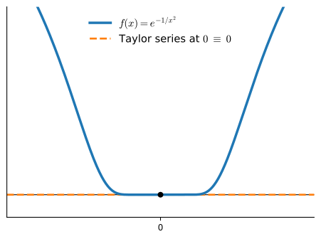
Two separate things can go wrong, which is why the definition demands both. The series can fail to converge away from \(x_0\); and even where it converges, its sum can differ from \(f\), since convergence of the series is not the same as convergence to \(f\). Being infinitely differentiable (smooth) guarantees neither. The classic counterexample is \(f(x) = e^{-1/x^2}\) (with \(f(0) = 0\)), which is smooth everywhere yet has \(f^{(n)}(0) = 0\) for every \(n\); its Taylor series at \(x_0 = 0\) is identically zero: it converges on the whole line, but to the zero function, reproducing \(f\) only at \(x = 0\) itself (Figure 25.1.10). So an infinite radius of convergence guarantees nothing about agreement with \(f\). In practice we mostly use the finite truncations \(P_n\), whose error Equation 25.1.7 we can bound directly, and which sharpen the closer \(x\) is to \(x_0\).
Take \(f(x) = e^{x}\) as an example. Since \(e^{x}\) is its own derivative, we know that \(f^{(n)}(x) = e^{x}\). Therefore, \(e^{x}\) can be reconstructed by taking the Taylor series at \(x_0 = 0\), i.e.,
\[ e^{x} = \sum_{n = 0}^\infty \frac{x^{n}}{n!} = 1 + x + \frac{x^2}{2} + \frac{x^3}{6} + \cdots. \]
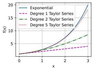
Plotting \(P_1\), \(P_2\), and \(P_5\) against \(e^x\) shows each higher degree tracking the curve farther from the base point.
# This calculation is backend-neutral, so one NumPy cell serves every tab.
xs = onp.arange(0, 3, 0.01)
ys = onp.exp(xs)
P1 = 1 + xs
P2 = 1 + xs + xs**2 / 2
P5 = 1 + xs + xs**2 / 2 + xs**3 / 6 + xs**4 / 24 + xs**5 / 120

d2l.plot(xs, [ys, P1, P2, P5], 'x', 'f(x)', legend=[
    "Exponential", "Degree 1 Taylor Series", "Degree 2 Taylor Series",
    "Degree 5 Taylor Series"])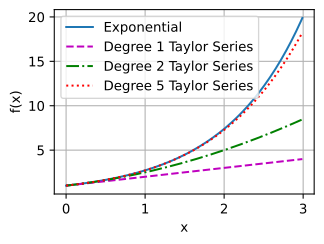
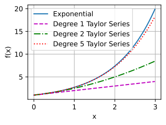
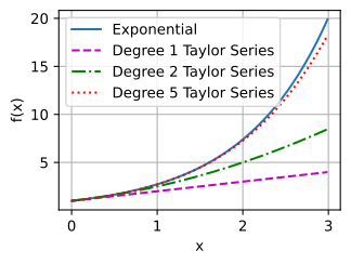
Taylor series matter here in two ways. Theoretically, replacing an unwieldy function by its low-degree polynomial makes it tractable: the first-order term is what gave us gradient descent, the second-order term is the curvature behind Newton’s method and step-size limits. Numerically, the same local-polynomial idea underlies elementary-function libraries, but production implementations do more than truncate the Taylor series at the input: they first reduce the argument to a small interval and then evaluate a carefully chosen polynomial or rational approximation with controlled error.
25.1.5 Nondifferentiable Points
The local linear approximation requires the limit in Equation 25.1.1 to exist. Functions such as \(|x|\) and \(\mathrm{ReLU}(x)=\max(0,x)\) have corners at the origin, where their left and right slopes differ. We examine one-sided derivatives, subgradients, and the treatment of such points in stochastic optimization (Section 9.3).
25.1.5.1 One-Sided Derivatives
The trouble is visible directly in the difference quotient Equation 25.1.1. For \(f(x) = |x|\) at \(x = 0\),
\[ \frac{|0+\epsilon| - |0|}{\epsilon} = \frac{|\epsilon|}{\epsilon} = \begin{cases} +1 & \epsilon > 0, \\ -1 & \epsilon < 0. \end{cases} \]
The two sides give different limits, so no single number is the slope: approaching from the right the function rises with slope \(+1\), from the left it falls with slope \(-1\). These are the one-sided derivatives \(f'_+(0) = +1\) and \(f'_-(0) = -1\). The ordinary two-sided derivative exists only when they agree. For \(\mathrm{ReLU}\) at \(0\) the same computation gives \(f'_-(0) = 0\) (flat on the left) and \(f'_+(0) = 1\) (slope \(1\) on the right). Note there is no limit to take: for \(|x|\) at \(0\) the two quotients are the constants \(\pm 1\), the same at every \(\epsilon\), so the next cell prints them once. It then evaluates what autograd returns at the corner, where no true derivative exists.
# One-sided difference quotients of |x| at 0: constants, no limit needed
epsilon = 1e-4
print(f'right quotient: {(abs(epsilon) - abs(0)) / epsilon:+.1f}, '
      f'left quotient: {(abs(-epsilon) - abs(0)) / -epsilon:+.1f}')

# What autograd returns at the corner, where no derivative exists
for name, fn in [('d|x|/dx', torch.abs), ("ReLU'", torch.relu)]:
    x = torch.tensor(0.0, requires_grad=True)
    fn(x).backward()
    print(f"{name} at 0: autograd returns {x.grad.item():.1f}")
right quotient: +1.0, left quotient: -1.0
d|x|/dx at 0: autograd returns 0.0
ReLU' at 0: autograd returns 0.0# One-sided difference quotients of |x| at 0: constants, no limit needed
epsilon = 1e-4
print(f'right quotient: {(abs(epsilon) - abs(0)) / epsilon:+.1f}, '
f'left quotient: {(abs(-epsilon) - abs(0)) / -epsilon:+.1f}')
# What autograd returns at the corner, where no derivative exists
for name, fn in [('d|x|/dx', tf.abs), ("ReLU'", tf.nn.relu)]:
x = tf.Variable(0.0)
with tf.GradientTape() as t:
y = fn(x)
print(f"{name} at 0: autograd returns {t.gradient(y, x).numpy():.1f}")right quotient: +1.0, left quotient: -1.0
d|x|/dx at 0: autograd returns 0.0
ReLU' at 0: autograd returns 0.0# One-sided difference quotients of |x| at 0: constants, no limit needed
epsilon = 1e-4
print(f'right quotient: {(abs(epsilon) - abs(0)) / epsilon:+.1f}, '
f'left quotient: {(abs(-epsilon) - abs(0)) / -epsilon:+.1f}')
# What autograd returns at the corner, where no derivative exists
for name, fn in [('d|x|/dx', jnp.abs), ("ReLU'", jax.nn.relu)]:
print(f"{name} at 0: autograd returns {jax.grad(fn)(0.0):.1f}")right quotient: +1.0, left quotient: -1.0
d|x|/dx at 0: autograd returns 1.0
ReLU' at 0: autograd returns 0.0# One-sided difference quotients of |x| at 0: constants, no limit needed
epsilon = 1e-4
print(f'right quotient: {(abs(epsilon) - abs(0)) / epsilon:+.1f}, '
f'left quotient: {(abs(-epsilon) - abs(0)) / -epsilon:+.1f}')
# What autograd returns at the corner, where no derivative exists
for name, fn in [('d|x|/dx', np.abs), ("ReLU'", npx.relu)]:
x = np.array(0.0)
x.attach_grad()
with autograd.record():
y = fn(x)
y.backward()
print(f"{name} at 0: autograd returns {float(x.grad):.1f}")right quotient: +1.0, left quotient: -1.0
d|x|/dx at 0: autograd returns 0.0
ReLU' at 0: autograd returns 0.0For both \(\frac{d}{dx}|x|\) and \(\mathrm{ReLU}'\) at \(0\) it returns the fixed value \(0\): one particular slope, chosen by convention, from the set of candidates we now define.
25.1.5.2 Subgradients and Optimality
The fix is to stop insisting on a single tangent and allow all the lines that stay below the graph. A number \(g\) is a subgradient of a convex function \(f\) (one whose every chord lies on or above its graph) at \(x\) if
\[ f(y) \ge f(x) + g\,(y - x) \quad \textrm{for all } y, \tag{25.1.8}\]
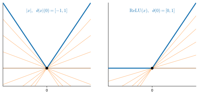
i.e. the line through \((x, f(x))\) with slope \(g\) is a global underestimate of \(f\). The set of all such slopes is the subdifferential \(\partial f(x)\) (Rockafellar 1970). Away from a corner it is the single ordinary slope; at a corner it is the whole interval between the one-sided derivatives, the “fan” of supporting lines shown in Figure 25.1.11:
\[ \partial |x|(0) = [-1, 1], \qquad \partial\, \mathrm{ReLU}(0) = [0, 1]. \]
Off the corner each function is differentiable and the subdifferential collapses to the single ordinary slope; at the corner, the \(0\) that autograd returned above is one element of each set.
The subgradient restores the optimality test. For differentiable \(f\) a minimum requires \(f'(x) = 0\); the subgradient version is the inclusion
\[ 0 \in \partial f(x). \tag{25.1.9}\]
This is no harder to prove than its smooth cousin: taking \(g = 0\) in Equation 25.1.8 reads \(f(y) \ge f(x)\) for all \(y\), which is precisely the statement that \(x\) is a global minimum. For \(|x|\) at \(0\) we have \(0 \in [-1,1] = \partial|x|(0)\), correctly certifying the origin as the minimum even though no derivative exists there, exactly the case the smooth test \(f'(x)=0\) cannot reach.
25.1.5.3 Nonsmooth Points in Stochastic Training
Nondifferentiable corners generally do not prevent stochastic training. The relevant behavior is the value that autograd assigns at each corner. One clarification first, so the convexity above is not over-read: a deep network’s loss surface is wildly non-convex, while the subdifferential Equation 25.1.8 is a convex-function notion. The kinks in a network come from convex building blocks (\(|x|\), \(\mathrm{ReLU}\), the hinge loss \(\max(0, 1-x)\)), and what autograd does at each kink is simple: it returns one fixed element of that piece’s subdifferential (the deep-learning libraries’ convention is \(\mathrm{ReLU}'(0) = 0\), as the cell above showed) and lets the chain rule propagate that choice through the surrounding, nonconvex composition.
Two caveats apply. First, even for a convex function a subgradient step need not be a descent step: at the minimum of \(|x|\) the perfectly valid subgradient \(g = \tfrac12 \in \partial|x|(0)\) sends the update to \(x = -\eta/2\) and increases the function; the subgradient method of convex optimization converges by shrinking its step sizes, not by descending monotonically (Nesterov 2018). Second, the chain rule carries no warranty at kinks: chaining per-kink choices can produce a number that is not a subgradient of the composite at all. The simplest failure is the identity in disguise
\[ g(x) = \mathrm{ReLU}(x) - \mathrm{ReLU}(-x) = x \quad \textrm{for all } x, \]
whose only correct slope at \(0\) is \(1\). The chain rule gives \(g'(x) = \mathrm{ReLU}'(x) + \mathrm{ReLU}'(-x)\), which is indeed \(1\) everywhere except at the kink, where the fixed convention makes it \(0 + 0 = 0\). The next cell runs exactly this computation.
# g(x) = relu(x) - relu(-x) is the identity, so the true slope at 0 is 1
x = torch.tensor(0.0, requires_grad=True)
g = torch.relu(x) - torch.relu(-x)
g.backward()
print(f"autograd: g'(0) = {x.grad.item():.1f}  (true slope: 1.0)")
autograd: g'(0) = 0.0 (true slope: 1.0)# g(x) = relu(x) - relu(-x) is the identity, so the true slope at 0 is 1
x = tf.Variable(0.0)
with tf.GradientTape() as t:
g = tf.nn.relu(x) - tf.nn.relu(-x)
print(f"autograd: g'(0) = {t.gradient(g, x).numpy():.1f} (true slope: 1.0)")autograd: g'(0) = 0.0 (true slope: 1.0)# g(x) = relu(x) - relu(-x) is the identity, so the true slope at 0 is 1
g = lambda x: jax.nn.relu(x) - jax.nn.relu(-x)
print(f"autograd: g'(0) = {jax.grad(g)(0.0):.1f} (true slope: 1.0)")autograd: g'(0) = 0.0 (true slope: 1.0)# g(x) = relu(x) - relu(-x) is the identity, so the true slope at 0 is 1
x = np.array(0.0)
x.attach_grad()
with autograd.record():
g = npx.relu(x) - npx.relu(-x)
g.backward()
print(f"autograd: g'(0) = {float(x.grad):.1f} (true slope: 1.0)")autograd: g'(0) = 0.0 (true slope: 1.0)Autograd reports slope \(0\) for a function that is the identity: the per-kink convention \(\mathrm{ReLU}'(0) = 0\), chained, produces a number that is not a subgradient of \(g\) at \(0\) at all. What automatic differentiation computes at nonsmooth points is, in general, an element of a conservative field (Bolte and Pauwels 2021), a relaxed gradient notion that agrees with the true derivative everywhere outside a measure-zero set, one so small it can be covered by intervals of arbitrarily small total length (Section 27.1 makes such size-zero statements precise). Rademacher’s theorem (Rademacher 1919) guarantees that a Lipschitz function even has a derivative outside a measure-zero set. Under the definability/path-differentiability assumptions studied by Bolte and Pauwels (2021), together with bounded iterates and the usual stochastic-approximation conditions on steps and gradient noise, SGD driven by such a conservative field converges to an appropriate stationary set almost surely. This is a conditional theorem, not a guarantee for every nonsmooth program.
Why does training tolerate the occasional bad chained value? The usual picture is that a network’s kinks (the points where some \(\mathrm{ReLU}\) input is exactly zero) form a measure-zero set, and a randomly drawn point lands in a measure-zero set with probability zero, provided the draw comes from a distribution with a density (an absolutely continuous one). Take this as a heuristic picture rather than a theorem: we have not proved that the kink set of a whole network is measure zero, and in floating-point arithmetic the argument fails outright, since the floats are a countable set on which every representable value, exact zeros included, carries positive probability. The rigorous result is the conservative-field convergence theorem quoted above; Section 9.2 develops the relevant convex analysis further. The local-linear approximation applies at almost every stochastic training step, where the function is smooth, and conservative-field theory covers the steps that land on a kink.
25.1.6 Summary
- The derivative is the local linear model of a function: \(f(x+\epsilon) \approx f(x) + \epsilon f'(x)\). It is the slope of the line a smooth curve flattens onto when we zoom in, and the limit of difference quotients.
- The derivatives of elementary functions, combined with the sum, product, and chain rules, differentiate any expression mechanically. Each rule is the small-change identity expanded to first order; the chain rule run in reverse over a network is backpropagation.
- Choosing the step \(\epsilon = -\eta f'(x)\) in the local model predicts a decrease of \(\eta[f'(x)]^2\). When the slope is \(L\)-Lipschitz the descent lemma turns this into a genuine guarantee \(f(x - \eta f'(x)) \le f(x) - \eta(1 - L\eta/2)[f'(x)]^2\), a strict drop for \(0 < \eta < 2/L\) (best at \(\eta = 1/L\)). Descent stalls at the stationary points \(f'(x) = 0\), and a step past \(2/L\) can increase \(f\) when curvature overwhelms the first-order gain.
- The second derivative is curvature: its sign decides minimum vs. maximum, and Taylor series extend the line and parabola to the best polynomial model of any order.
- At corners like \(\mathrm{ReLU}(0)\) the derivative is undefined, but the subdifferential supplies a set of valid slopes (\(\partial|x|(0) = [-1,1]\)) and optimality becomes \(0 \in \partial f(x)\). Autograd returns one fixed element per kink (\(\mathrm{ReLU}'(0) = 0\)); chained through a composition that value can fail to be a subgradient at the kinks themselves. Conservative-field theory supplies convergence results under additional structural, boundedness, step-size, and noise assumptions.
25.1.7 Exercises
- Compute the derivative of \(x^3 - 4x + 1\), and of \(\log\!\left(\frac{1}{x}\right)\) for \(x > 0\).
- Derive the quotient rule from the product and chain rules by writing \(\frac{g(x)}{h(x)} = g(x)\cdot\left(h(x)\right)^{-1}\) and using the power rule with \(n = -1\) for the outer function. Check your result on \(\tan(x) = \frac{\sin(x)}{\cos(x)}\): you should find \(\frac{d}{dx}\tan(x) = \frac{1}{\cos^2(x)}\).
- True or false: if \(f'(x) = 0\) then \(f\) has a maximum or a minimum at \(x\). If false, give a counterexample and the test that distinguishes the cases.
- Find the minimum of \(f(x) = x\log(x)\) for \(x \ge 0\) (take the limiting value \(f(0) = 0\)).
- The first-order model predicts \(f(x - \eta f'(x)) \approx f(x) - \eta[f'(x)]^2\). Starting from the small-change identity, derive this prediction and name the term it discards. Then extend the descent lemma to the vector case: for \(f: \mathbb{R}^n \to \mathbb{R}\) with an \(L\)-Lipschitz gradient (\(\|\nabla f(\mathbf{u}) - \nabla f(\mathbf{v})\| \le L\|\mathbf{u} - \mathbf{v}\|\)), show that \(f(\mathbf{x} - \eta\nabla f(\mathbf{x})) \le f(\mathbf{x}) - \eta\left(1 - \tfrac{L\eta}{2}\right)\|\nabla f(\mathbf{x})\|^2\). (Hint: repeat the proof of Equation 25.1.3 along the segment \(\mathbf{x} + t\mathbf{s}\) with \(\mathbf{s} = -\eta\nabla f(\mathbf{x})\), bounding the integral with the Cauchy–Schwarz inequality.)
- For \(f(x) = x^2\), find all step sizes \(\eta\) for which gradient descent from \(x_0 \neq 0\) converges to the minimum, and the one \(\eta\) that reaches it in a single step. (Hint: use \(x_{t+1} = (1-2\eta)x_t\).)
- Give a function \(f\) and a step size \(\eta\) for which a single gradient-descent step increases \(f\), and explain the failure: which hypothesis of the descent lemma Equation 25.1.3 is violated, or is \(\eta\) simply past \(2/L\)? (Hint: \(f(x) = x^2\) with \(\eta > 1\) already does it.)
- Relate the one-dimensional update \(x \leftarrow x - \eta f'(x)\) to the vector update \(\mathbf{w} \leftarrow \mathbf{w} - \eta\nabla L(\mathbf{w})\) from the introduction.
- Compute the subdifferentials \(\partial\,\mathrm{ReLU}(0)\) and \(\partial|x|(0)\). Which of \(\{0,\, 0.5,\, 1\}\) are valid subgradients of \(\mathrm{ReLU}\) at \(0\)? Sketch the subdifferential of the hinge loss \(\max(0, 1 - x)\).
- Use the degree-\(5\) Taylor polynomial of \(e^x\) at \(x_0 = 0\) to estimate \(e\), and compare with the true value.