%matplotlib inline
from d2l import torch as d2l
import numpy as np15.3 Regularized Policy Optimization
PPO constrains each policy update relative to the preceding policy. A different objective keeps the policy near a fixed reference by subtracting a KL-divergence penalty from expected reward. This changes the optimum, not only the path taken by the optimizer, and it includes entropy regularization as the special case of a uniform reference.
We first examine why such a reference can be useful when rewards are learned from preferences. A reward model is accurate only where its comparison data provide information, and optimizing it can exploit errors elsewhere. A tabular gridworld makes this failure measurable against the true reward. We then derive the KL-regularized optimum, its soft Bellman backup, and its connections to language-model post-training and maximum-entropy reinforcement learning.
%matplotlib inline
from d2l import jax as d2l
import numpy as np
15.3.1 Learning Rewards from Preferences
For many tasks, such as evaluating a helpful answer or a safe driving maneuver, an explicit numerical reward is difficult to specify. Pairwise comparisons are often easier to obtain. Preference-based reinforcement learning fits a reward model to these comparisons and then optimizes the learned reward (Christiano et al. 2017). We represent the comparison model with logistic regression.
15.3.1.1 Preferences and the Bradley-Terry Model
The Bradley-Terry model (Bradley and Terry 1952) assigns each candidate a scalar score, here the return of a trajectory, and models a comparison as a noisy observation of the score difference:
\[P(\tau \succ \tau') = \sigma\big( r(\tau) - r(\tau') \big), \qquad \sigma(u) = \frac{1}{1 + e^{-u}}. \tag{15.3.1}\]
Fitting \(r\) by maximum likelihood on labeled pairs is logistic regression on feature differences. We use a \(4 \times 4\) gridworld with deterministic moves, an absorbing goal in the far corner worth \(+1\), a living cost of \(-0.04\) per step, and two central hazard cells that cost \(-1.5\) to enter. The reference policy \(\pi_{\textrm{ref}}\) is a softmax over the true action values at temperature \(0.25\). It reaches the goal but remains stochastic, and it rarely enters the hazard lane.
gamma = 0.95                                   # a 4 x 4 gridworld
P = np.zeros((16, 4, 16))
for s, a in np.ndindex(16, 4):
    x, y = s % 4, s // 4
    dx, dy = [(-1, 0), (0, 1), (1, 0), (0, -1)][a]   # left, down, right, up
    P[s, a, min(3, max(0, y + dy)) * 4 + min(3, max(0, x + dx))] = 1.0
P[15], P[15, :, 15] = 0.0, 1.0                 # the goal absorbs
bonus = np.full(16, -0.04)                     # every step costs a little
bonus[[5, 6]], bonus[15] = -1.5, 1.0           # a hazard lane; the goal pays
r_true = np.einsum('sat,t->sa', P, bonus)      # r*(s, a): the entered bonus
r_true[15] = 0.0
mdp = d2l.TabularMDP(P, r_true, gamma)
Q_true = mdp.backup(d2l.value_iteration(mdp, 200)[-1])
pi_ref = np.exp(Q_true / 0.25)                 # competent but hedging
pi_ref /= pi_ref.sum(1, keepdims=True)
gamma = 0.95 # a 4 x 4 gridworld
P = np.zeros((16, 4, 16))
for s, a in np.ndindex(16, 4):
x, y = s % 4, s // 4
dx, dy = [(-1, 0), (0, 1), (1, 0), (0, -1)][a] # left, down, right, up
P[s, a, min(3, max(0, y + dy)) * 4 + min(3, max(0, x + dx))] = 1.0
P[15], P[15, :, 15] = 0.0, 1.0 # the goal absorbs
bonus = np.full(16, -0.04) # every step costs a little
bonus[[5, 6]], bonus[15] = -1.5, 1.0 # a hazard lane; the goal pays
r_true = np.einsum('sat,t->sa', P, bonus) # r*(s, a): the entered bonus
r_true[15] = 0.0
mdp = d2l.TabularMDP(P, r_true, gamma)
Q_true = mdp.backup(d2l.value_iteration(mdp, 200)[-1])
pi_ref = np.exp(Q_true / 0.25) # competent but hedging
pi_ref /= pi_ref.sum(1, keepdims=True)We next withhold \(r^*\) and estimate it from comparisons. We collect one thousand trajectories from \(\pi_{\textrm{ref}}\) and represent each by its discounted visit counts \(x(\tau)\), for which the true return is \(x(\tau)^\top r^*\). We sample six thousand pairs, label them according to Equation 15.3.1, and fit \(\hat r\) by logistic regression on feature differences. A stated weight-decay coefficient regularizes this finite diagnostic:
rng = np.random.default_rng(0)

def sample_traj(pi, T=40):
    s, x = 0, np.zeros((16, 4))
    for t in range(T):
        a = rng.choice(4, p=pi[s])
        x[s, a] += gamma ** t                  # discounted visits: R = x . r
        s = P[s, a].argmax()
        if s == 15:
            break
    return x.ravel()

X = np.stack([sample_traj(pi_ref) for _ in range(1000)])
R = X @ r_true.ravel()                         # true returns; the fit never sees them
i, j = rng.integers(0, 1000, (2, 6000))
y = (rng.random(6000) < 1 / (1 + np.exp(R[j] - R[i]))).astype(float)
D = X[i] - X[j]
w = np.zeros(64)
for _ in range(4000):                          # logistic regression on (D, y)
    w += 0.5 * (D.T @ (y - 1 / (1 + np.exp(-D @ w))) / len(y) - 0.02 * w)
r_hat = w.reshape(16, 4)
core = (X > 0).sum(0).reshape(16, 4) >= 50     # pairs seen in >= 50 episodes
print(f'never visited: {(X.sum(0) == 0).sum()} pairs; '
      f'in at least 50 episodes: {core.sum()} pairs')
print(f'rms fit error on those {core.sum()}: '
      f'{np.sqrt(((r_hat - r_true)[core] ** 2).mean()):.3f}')
print(f'entries into the hazard lane: true '
      f'{np.round(r_true[[1, 4, 2, 5], [1, 2, 1, 2]], 2)}, '
      f'fitted {np.round(r_hat[[1, 4, 2, 5], [1, 2, 1, 2]], 2)}')
never visited: 9 pairs; in at least 50 episodes: 46 pairs
rms fit error on those 46: 0.193
entries into the hazard lane: true [-1.5 -1.5 -1.5 -1.5], fitted [-0.03 -0.05 -0.02 0. ]rng = np.random.default_rng(0)
def sample_traj(pi, T=40):
s, x = 0, np.zeros((16, 4))
for t in range(T):
a = rng.choice(4, p=pi[s])
x[s, a] += gamma ** t # discounted visits: R = x . r
s = P[s, a].argmax()
if s == 15:
break
return x.ravel()
X = np.stack([sample_traj(pi_ref) for _ in range(1000)])
R = X @ r_true.ravel() # true returns; the fit never sees them
i, j = rng.integers(0, 1000, (2, 6000))
y = (rng.random(6000) < 1 / (1 + np.exp(R[j] - R[i]))).astype(float)
D = X[i] - X[j]
w = np.zeros(64)
for _ in range(4000): # logistic regression on (D, y)
w += 0.5 * (D.T @ (y - 1 / (1 + np.exp(-D @ w))) / len(y) - 0.02 * w)
r_hat = w.reshape(16, 4)
core = (X > 0).sum(0).reshape(16, 4) >= 50 # pairs seen in >= 50 episodes
print(f'never visited: {(X.sum(0) == 0).sum()} pairs; '
f'in at least 50 episodes: {core.sum()} pairs')
print(f'rms fit error on those {core.sum()}: '
f'{np.sqrt(((r_hat - r_true)[core] ** 2).mean()):.3f}')
print(f'entries into the hazard lane: true '
f'{np.round(r_true[[1, 4, 2, 5], [1, 2, 1, 2]], 2)}, '
f'fitted {np.round(r_hat[[1, 4, 2, 5], [1, 2, 1, 2]], 2)}')never visited: 9 pairs; in at least 50 episodes: 46 pairs
rms fit error on those 46: 0.193
entries into the hazard lane: true [-1.5 -1.5 -1.5 -1.5], fitted [-0.03 -0.05 -0.02 0. ]The fit has an rms error of \(0.19\) on the forty-six state-action pairs visited by the reference policy. Nine pairs are absent from the data, so their fitted rewards remain at the initialization value of zero. This matters for the hazard lane: entering it has true reward \(-1.5\), but the fitted model assigns a value near zero because the reference policy rarely provides comparisons there. In this example, zero initialization and weight decay make unsupported predictions remain near zero. A neural reward model need not behave this way and may extrapolate unpredictably outside the data distribution.
15.3.1.2 Identifiability and the Per-Prompt Baseline
A comparison includes two trajectories from the same start state, so Equation 15.3.1 depends only on score differences. In the prompt-response notation used at scale, shifting the reward by any function of the prompt, \(r(x, y) \to r(x, y) + f(x)\), leaves every difference and therefore the likelihood unchanged; exercise 5 asks you to verify this result. A learned reward is thus identified only relative to each prompt, and its absolute level per prompt is a convention. Subtracting a per-prompt baseline does not change the comparison model. Independently, the zero-mean lemma of Section 14.6 shows that subtracting any function of the state from the policy-gradient weight preserves unbiasedness. The group mean used by GRPO (Section 14.6) combines these two properties, subject to the self-inclusion qualification developed later.
15.3.1.3 Dense versus Terminal Rewards
Our comparisons score complete trajectories, so \(\hat r\) is trained on end-to-end evidence. At scale, an outcome reward model (ORM) likewise scores a completed response, whereas a process reward model (PRM) scores intermediate steps. Intermediate rewards provide denser credit-assignment signals but require additional labels and introduce more opportunities for misspecification. Potential-based shaping is the standard densification that preserves the optimal policy under its stated conditions (Ng et al. 1999).
15.3.2 Optimizing a Proxy Reward
We now optimize \(\hat{r}\) directly with value iteration.
15.3.2.1 Reward Hacking and Goodhart’s Law
Goodhart’s law describes the loss of validity that can occur when a measure becomes an optimization target. In reinforcement learning, reward hacking denotes policies that score highly under a specified or fitted reward while violating the intended objective; many examples are catalogued in (Krakovna et al. 2020). The shaped-bonus example in Section 14.1 had the same mechanism: optimization uses errors in the estimated objective. There the error was specified manually; here it is statistical. We plan optimally under \(\hat{r}\) with value iteration (Section 14.2) and evaluate the resulting policy under \(r^*\):
def plan(r):
    m = d2l.TabularMDP(P, r, gamma)
    return np.eye(4)[m.backup(d2l.value_iteration(m, 200)[-1]).argmax(1)]

def ret(pi, r):
    m = d2l.TabularMDP(P, r, gamma)
    return d2l.policy_evaluation(m, pi, 400)[-1][0]

for name, r in (('true reward  ', r_true), ('fitted reward', r_hat)):
    pi = plan(r)
    print(f'plan on {name}: fitted return {ret(pi, r_hat):+.2f}, '
          f'true return {ret(pi, r_true):+.2f}')
plan on true reward : fitted return -0.24, true return +0.59
plan on fitted reward: fitted return -0.03, true return -2.11def plan(r):
m = d2l.TabularMDP(P, r, gamma)
return np.eye(4)[m.backup(d2l.value_iteration(m, 200)[-1]).argmax(1)]
def ret(pi, r):
m = d2l.TabularMDP(P, r, gamma)
return d2l.policy_evaluation(m, pi, 400)[-1][0]
for name, r in (('true reward ', r_true), ('fitted reward', r_hat)):
pi = plan(r)
print(f'plan on {name}: fitted return {ret(pi, r_hat):+.2f}, '
f'true return {ret(pi, r_true):+.2f}')plan on true reward : fitted return -0.24, true return +0.59
plan on fitted reward: fitted return -0.03, true return -2.11Under the fitted reward, the optimized policy scores \(-0.03\), compared with \(-0.24\) for the reference policy; only the difference is meaningful because the additive reward constant is unidentified. Under the true reward, however, the scores are \(-2.11\) and \(+0.59\). The optimized policy enters the hazard lane because its unsupported rewards were estimated near zero. Value iteration has optimized the supplied reward correctly; the failure lies in the reward model outside the reference policy’s data distribution. Section 15.6 encounters the same problem for learned value functions.
15.3.2.2 True Return against the KL Budget
The available evidence supports \(\hat{r}\) primarily on trajectories sampled from \(\pi_{\textrm{ref}}\). We therefore measure policy displacement from the reference with the KL divergence. For each coefficient \(\beta\), we compute the policy that maximizes \(\sum_t \gamma^t \big( \hat{r}_t - \beta\, D_{\textrm{KL}}( \pi(\cdot \mid s_t) \Vert \pi_{\textrm{ref}}(\cdot \mid s_t) ) \big)\), thereby tracing fitted and true return as functions of divergence. The next section derives this objective for a single decision and proves its optimum in closed form; in an MDP the optimum must also account for every later step’s reward and penalty, and it does so through a \(\beta\)-dependent soft action value: replace value iteration’s hard-max backup (Section 14.2) with the reference-weighted soft one,
\[V_\beta(s) = \beta \log \sum_a \pi_{\textrm{ref}}(a \mid s)\, e^{Q_\beta(s, a)/\beta}, \qquad Q_\beta(s, a) = \hat{r}(s, a) + \gamma \sum_{s'} P(s' \mid s, a)\, V_\beta(s'),\]
whose fixed point gives the exactly optimal policy \(\pi_\beta(a \mid s) \propto \pi_{\textrm{ref}}(a \mid s)\, e^{Q_\beta(s, a)/\beta}\). The next section derives this backup. Like the ordinary Bellman backup of Section 14.2, it is a contraction, and the loop below solves its fixed point for each \(\beta\). The printed residual measures numerical convergence. Large \(\beta\) keeps the policy close to the reference, whereas small \(\beta\) approaches the fitted-reward maximizer. For each \(\pi_\beta\), we record true return, fitted return, and the discounted sum of per-state divergences from the reference along trajectories generated by \(\pi_\beta\):
def soft_v(r, beta, num_iters=400):
    """Soft value iteration for the KL-penalized objective: iterate
    V(s) <- beta log sum_a pi_ref(a|s) exp((r + gamma P V)(s, a) / beta)."""
    V = np.zeros(16)
    for _ in range(num_iters):
        Q = r + gamma * np.einsum('sat,t->sa', P, V)
        m = Q.max(1)
        V = m + beta * np.log(
            (pi_ref * np.exp((Q - m[:, None]) / beta)).sum(1))
    return V

kls, true_ret, prox_ret, resid = [], [], [], 0.0
for beta in np.logspace(1, -2.5, 36):
    V_b = soft_v(r_hat, beta)
    Q_b = r_hat + gamma * np.einsum('sat,t->sa', P, V_b)
    m = Q_b.max(1, keepdims=True)
    pi = pi_ref * np.exp((Q_b - m) / beta)     # the exact optimum: pi_ref
    pi /= pi.sum(1, keepdims=True)             # tilted by the soft Q_beta
    back = m[:, 0] + beta * np.log(
        (pi_ref * np.exp((Q_b - m) / beta)).sum(1))
    resid = max(resid, np.abs(back - V_b).max())   # Bellman residual
    kl = (pi * np.log(np.where(pi > 0, pi / pi_ref, 1.0))).sum(1)
    kl[15] = 0.0                               # no decisions once absorbed
    rho = np.linalg.solve(np.eye(16) - gamma
                          * np.einsum('sa,sat->st', pi, P).T, np.eye(16)[0])
    kls.append(rho @ kl)
    true_ret.append(ret(pi, r_true))
    prox_ret.append(ret(pi, r_hat))
k = int(np.argmax(true_ret))
print(f'largest soft Bellman residual across the sweep: {resid:.1e}')
print(f'true return {true_ret[0]:+.2f} at KL 0, peak {true_ret[k]:+.2f} '
      f'at KL {kls[k]:.1f}, then {true_ret[-1]:+.2f} at KL {kls[-1]:.1f}')
d2l.plot(kls, [true_ret, prox_ret], 'KL from the reference (nats)', 'return',
         legend=['true return', 'fitted return'])
largest soft Bellman residual across the sweep: 0.0e+00
true return -0.10 at KL 0, peak +0.53 at KL 3.7, then -1.83 at KL 14.2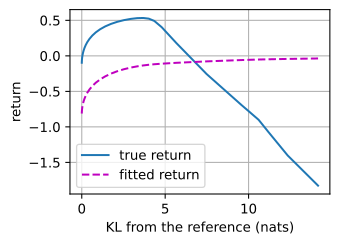
def soft_v(r, beta, num_iters=400):
    """Soft value iteration for the KL-penalized objective: iterate
    V(s) <- beta log sum_a pi_ref(a|s) exp((r + gamma P V)(s, a) / beta)."""
    V = np.zeros(16)
    for _ in range(num_iters):
        Q = r + gamma * np.einsum('sat,t->sa', P, V)
        m = Q.max(1)
        V = m + beta * np.log(
            (pi_ref * np.exp((Q - m[:, None]) / beta)).sum(1))
    return V

kls, true_ret, prox_ret, resid = [], [], [], 0.0
for beta in np.logspace(1, -2.5, 36):
    V_b = soft_v(r_hat, beta)
    Q_b = r_hat + gamma * np.einsum('sat,t->sa', P, V_b)
    m = Q_b.max(1, keepdims=True)
    pi = pi_ref * np.exp((Q_b - m) / beta)     # the exact optimum: pi_ref
    pi /= pi.sum(1, keepdims=True)             # tilted by the soft Q_beta
    back = m[:, 0] + beta * np.log(
        (pi_ref * np.exp((Q_b - m) / beta)).sum(1))
    resid = max(resid, np.abs(back - V_b).max())   # Bellman residual
    kl = (pi * np.log(np.where(pi > 0, pi / pi_ref, 1.0))).sum(1)
    kl[15] = 0.0                               # no decisions once absorbed
    rho = np.linalg.solve(np.eye(16) - gamma
                          * np.einsum('sa,sat->st', pi, P).T, np.eye(16)[0])
    kls.append(rho @ kl)
    true_ret.append(ret(pi, r_true))
    prox_ret.append(ret(pi, r_hat))
k = int(np.argmax(true_ret))
print(f'largest soft Bellman residual across the sweep: {resid:.1e}')
print(f'true return {true_ret[0]:+.2f} at KL 0, peak {true_ret[k]:+.2f} '
      f'at KL {kls[k]:.1f}, then {true_ret[-1]:+.2f} at KL {kls[-1]:.1f}')
d2l.plot(kls, [true_ret, prox_ret], 'KL from the reference (nats)', 'return',
         legend=['true return', 'fitted return'])
largest soft Bellman residual across the sweep: 0.0e+00
true return -0.10 at KL 0, peak +0.53 at KL 3.7, then -1.83 at KL 14.2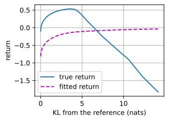
Every point in this figure is an optimum of the penalized objective; the Bellman residual is zero to double precision. The fitted return increases throughout the sweep. The true return instead rises from \(-0.10\) to \(+0.53\) at a divergence just below four nats, and then decreases sharply as the policy concentrates on the hazard lane. Moderate optimization of the imperfect reward model improves the true return, whereas further optimization exploits its unsupported predictions. A similar nonmonotonic relation has been observed when language models are optimized against a learned reward and evaluated by a separate reference measure (Gao et al. 2023). This motivates controlling the divergence from the reference policy directly.
15.3.3 The Regularized Objective
Whereas Chapter 14 maximized expected reward, a fixed-reference penalty can restrict optimization of a learned reward to policies near the data-generating policy. For a single decision with reward \(r(a)\) over a finite action set, reference \(\pi_{\textrm{ref}}\), and coefficient \(\beta > 0\), the regularized objective is
\[\max_{\pi}\ E_{a \sim \pi}\big[ r(a) \big] - \beta\, D_{\textrm{KL}}\big( \pi \Vert \pi_{\textrm{ref}} \big). \tag{15.3.2}\]
The penalty is part of the objective rather than a constraint on a single update. The coefficient \(\beta\) sets its weight relative to reward, and the reference policy remains fixed.
15.3.3.1 The Closed-Form Optimum
Proposition. For \(\beta > 0\), the objective Equation 15.3.2 is maximized by the unique policy
\[\pi^\star(a) = \frac{1}{Z}\, \pi_{\textrm{ref}}(a)\, e^{r(a)/\beta}, \qquad Z = \sum_{a} \pi_{\textrm{ref}}(a)\, e^{r(a)/\beta}, \tag{15.3.3}\]
and the maximal value is \(\beta \log Z\).
Proof. By construction \(r(a) = \beta \log\big( \pi^\star(a) Z / \pi_{\textrm{ref}}(a) \big)\). Substituting into the objective, for any policy \(\pi\),
\[E_\pi[r] - \beta D_{\textrm{KL}}(\pi \Vert \pi_{\textrm{ref}}) = \sum_a \pi(a)\, \beta \log \frac{\pi^\star(a)\, Z}{\pi(a)} = \beta \log Z - \beta\, D_{\textrm{KL}}(\pi \Vert \pi^\star).\]
Gibbs’ inequality, proved in Chapter 28, says the remaining divergence is nonnegative and zero exactly when \(\pi = \pi^\star\). \(\blacksquare\)
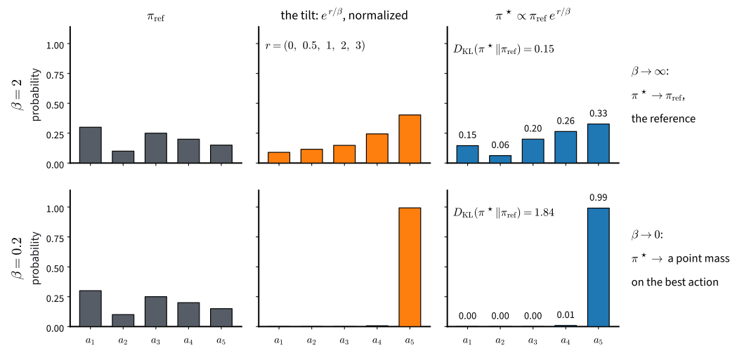
The optimum multiplies the reference by an exponential tilt and then renormalizes it, and the achieved value is a log-partition function. Figure 15.3.1 illustrates this relation. Two boundary cases complete the statement. The optimum inherits the reference’s support: if \(\pi_{\textrm{ref}}(a) = 0\), any policy placing mass on \(a\) has infinite divergence, so Equation 15.3.3 correctly assigns \(a\) zero probability, and no finite reward can assign positive probability to an action excluded by the reference. And as \(\beta \to 0\) the limit is a point mass only when the best action is unique; with ties, it is the reference renormalized over the maximizing set. We verify the proposition numerically by solving Equation 15.3.2 with exponentiated gradient ascent, using multiplicative updates renormalized onto the simplex; the \(+1\) in the exact gradient \(r - \beta(\log(\pi/\pi_{\textrm{ref}}) + 1)\) is constant across actions and cancels during normalization, so we drop it:
p_ref = np.array([0.30, 0.10, 0.25, 0.20, 0.15])
r = np.array([0.0, 0.5, 1.0, 2.0, 3.0])

def solve_kl(r, p, beta, steps=3000, eta=0.3):
    pi = np.full_like(p, 1 / len(p))
    for _ in range(steps):                     # exponentiated gradient ascent
        pi = pi * np.exp(eta * (r - beta * np.log(pi / p)))
        pi /= pi.sum()
    return pi

for beta in (5.0, 2.0, 0.5, 0.2):
    pi = solve_kl(r, p_ref, beta)
    print(f'beta = {beta:3}: pi_beta = {np.round(pi, 3)}, '
          f'reward {pi @ r:.2f}, KL {(pi * np.log(pi / p_ref)).sum():.2f}')
beta = 5.0: pi_beta = [0.233 0.086 0.237 0.232 0.212], reward 1.38, KL 0.02
beta = 2.0: pi_beta = [0.146 0.062 0.2 0.264 0.327], reward 1.74, KL 0.15
beta = 0.5: pi_beta = [0.004 0.004 0.025 0.148 0.819], reward 2.78, KL 1.26
beta = 0.2: pi_beta = [0. 0. 0. 0.009 0.991], reward 2.99, KL 1.84p_ref = np.array([0.30, 0.10, 0.25, 0.20, 0.15])
r = np.array([0.0, 0.5, 1.0, 2.0, 3.0])
def solve_kl(r, p, beta, steps=3000, eta=0.3):
pi = np.full_like(p, 1 / len(p))
for _ in range(steps): # exponentiated gradient ascent
pi = pi * np.exp(eta * (r - beta * np.log(pi / p)))
pi /= pi.sum()
return pi
for beta in (5.0, 2.0, 0.5, 0.2):
pi = solve_kl(r, p_ref, beta)
print(f'beta = {beta:3}: pi_beta = {np.round(pi, 3)}, '
f'reward {pi @ r:.2f}, KL {(pi * np.log(pi / p_ref)).sum():.2f}')beta = 5.0: pi_beta = [0.233 0.086 0.237 0.232 0.212], reward 1.38, KL 0.02
beta = 2.0: pi_beta = [0.146 0.062 0.2 0.264 0.327], reward 1.74, KL 0.15
beta = 0.5: pi_beta = [0.004 0.004 0.025 0.148 0.819], reward 2.78, KL 1.26
beta = 0.2: pi_beta = [0. 0. 0. 0.009 0.991], reward 2.99, KL 1.84Then compare against Equation 15.3.3, closed form against converged iterate, and the value against \(\beta \log Z\):
def pi_star(r, p, beta):
    star = p * np.exp((r - r.max()) / beta)    # eq_kl_optimum, stabilized
    return star / star.sum()

gap = max(np.abs(solve_kl(r, p_ref, b) - pi_star(r, p_ref, b)).max()
          for b in (5.0, 2.0, 0.5, 0.2))
pi2 = solve_kl(r, p_ref, 2.0)
print(f'largest gap to the closed form over the ladder: {gap:.1e}')
print(f'objective at beta = 2: numerical '
      f'{pi2 @ r - 2.0 * (pi2 * np.log(pi2 / p_ref)).sum():.6f}, '
      f'beta log Z = {2.0 * np.log(p_ref @ np.exp(r / 2.0)):.6f}')
largest gap to the closed form over the ladder: 1.4e-16
objective at beta = 2: numerical 1.442004, beta log Z = 1.442004def pi_star(r, p, beta):
star = p * np.exp((r - r.max()) / beta) # eq_kl_optimum, stabilized
return star / star.sum()
gap = max(np.abs(solve_kl(r, p_ref, b) - pi_star(r, p_ref, b)).max()
for b in (5.0, 2.0, 0.5, 0.2))
pi2 = solve_kl(r, p_ref, 2.0)
print(f'largest gap to the closed form over the ladder: {gap:.1e}')
print(f'objective at beta = 2: numerical '
f'{pi2 @ r - 2.0 * (pi2 * np.log(pi2 / p_ref)).sum():.6f}, '
f'beta log Z = {2.0 * np.log(p_ref @ np.exp(r / 2.0)):.6f}')largest gap to the closed form over the ladder: 1.4e-16
objective at beta = 2: numerical 1.442004, beta log Z = 1.442004Across the tested values of \(\beta\), the largest disagreement is at floating-point resolution, and the achieved objective matches \(\beta \log Z\) to six decimal places. This confirms the exact finite-action result numerically.
15.3.3.2 Four Consequences of the Closed Form
Without the penalty, the optimum is a point mass. Send \(\beta \to 0\) in Equation 15.3.3 and all mass flows to the highest-reward action, or, under ties, to the reference’s distribution over the tied set; that is just the unregularized problem, whose solution was always the argmax. This result characterizes the optimum, not the dynamics of a particular training run. The entropy decrease measured in Section 15.2 is consistent with movement toward the deterministic optimum of the unregularized objective. Regularization can instead make a stochastic policy optimal.
The coefficient controls the interpolation. The closed form gives the following limiting cases:
for beta in (100.0, 0.01):
    print(f'beta = {beta:6}: pi_star = {np.round(pi_star(r, p_ref, beta), 3)}')
beta = 100.0: pi_star = [0.297 0.099 0.25 0.202 0.153]
beta = 0.01: pi_star = [0. 0. 0. 0. 1.]for beta in (100.0, 0.01):
print(f'beta = {beta:6}: pi_star = {np.round(pi_star(r, p_ref, beta), 3)}')beta = 100.0: pi_star = [0.297 0.099 0.25 0.202 0.153]
beta = 0.01: pi_star = [0. 0. 0. 0. 1.]\(\beta \to \infty\) reproduces the reference; \(\beta \to 0\) is greedy; every policy between is an exact optimum of some exchange rate between reward and divergence.
A uniform reference is the entropy bonus. Against a uniform reference, \(D_{\textrm{KL}}(\pi \Vert \textrm{uniform}) = \log |\mathcal{A}| - H(\pi)\), so the penalty is an entropy bonus up to a constant, and Equation 15.3.2 becomes the maximum-entropy objective. The closed form specializes to a softmax of the reward:
boltzmann = np.exp(r / 0.5) / np.exp(r / 0.5).sum()
print(np.allclose(pi_star(r, np.full(5, 0.2), 0.5), boltzmann))Trueboltzmann = np.exp(r / 0.5) / np.exp(r / 0.5).sum()
print(np.allclose(pi_star(r, np.full(5, 0.2), 0.5), boltzmann))TrueThis is the form of Section 14.5’s softmax policies. The Boltzmann exploration distribution in Section 14.4 is also the optimizer of an entropy-regularized one-step objective, with temperature corresponding to \(\beta\). The sequential version of this consequence is the soft backup, which closes the section.
A posterior interpretation. Equation Equation 15.3.3 has the form of Bayes’ rule: \(\pi_{\textrm{ref}}\) is a prior, \(e^{r/\beta}\) an unnormalized likelihood, \(\pi^\star\) a posterior, and \(Z\) the normalizer. Control-as-inference methods use this identity to interpret rewards as log-likelihoods of optimality events and regularized policy optimization as variational inference (Levine 2018; Korbak et al. 2022). The analogy permits selected inference tools, but it does not by itself establish their approximation quality or empirical advantage for policies.
Sweeping \(\beta\) traces the exact reward–divergence frontier for the finite-action example. The gridworld experiment evaluates an analogous frontier using the imperfect estimate \(\hat{r}\):
front = np.stack([pi_star(r, p_ref, b) for b in np.logspace(1.5, -1.5, 61)])
kl_f = (front * np.log(front / p_ref)).sum(1)
print(f'KL 0 pays {p_ref @ r:.2f}; the frontier ends at KL '
      f'{np.log(1 / p_ref[r.argmax()]):.2f}, reward {r.max():.0f}')
d2l.plot(kl_f, front @ r, 'KL from the reference (nats)', 'expected reward')
KL 0 pays 1.15; the frontier ends at KL 1.90, reward 3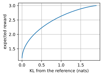
front = np.stack([pi_star(r, p_ref, b) for b in np.logspace(1.5, -1.5, 61)])
kl_f = (front * np.log(front / p_ref)).sum(1)
print(f'KL 0 pays {p_ref @ r:.2f}; the frontier ends at KL '
      f'{np.log(1 / p_ref[r.argmax()]):.2f}, reward {r.max():.0f}')
d2l.plot(kl_f, front @ r, 'KL from the reference (nats)', 'expected reward')
KL 0 pays 1.15; the frontier ends at KL 1.90, reward 3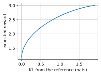
With true reward on the vertical axis, the frontier is concave and increasing (exercise 2), so its marginal reward gain per nat decreases. The gridworld curve is nonmonotonic because optimization uses the fitted reward while evaluation uses true return. The two rows of Figure 15.3.1 are two points on this curve.
15.3.3.3 Trust Region versus Penalty
Trust-region and fixed-reference methods both use KL divergence but in different roles.
Two uses of KL divergence. A trust region (Section 15.2) measures divergence from the previous iterate. It restricts each update and protects a local approximation, while its reference changes after the update. A fixed-reference penalty (this section) is part of the objective and changes the optimum to Equation 15.3.3. PPO-style language-model fine-tuning can use both: a clipped surrogate relative to the sampling policy for update stability, and a reward penalty relative to the frozen initial model to control the final policy (Ouyang et al. 2022).
15.3.3.4 The Direction of the KL Divergence
\(D_{\textrm{KL}}(\pi \Vert \pi_{\textrm{ref}})\) is the reverse divergence in the taxonomy of Section 28.2.2.2. Because it is an expectation under \(\pi\), it can be estimated from policy samples. It penalizes assigning probability where the reference has little support but does not penalize assigning zero probability to reference modes, producing mode-seeking behavior. The forward direction \(D_{\textrm{KL}}(\pi_{\textrm{ref}} \Vert \pi)\) instead penalizes failure to cover behavior sampled by the reference. The direction is therefore a modeling choice with different coverage effects.
15.3.4 The Soft Backup and Its Consequences
15.3.4.1 Maximum-Entropy Reinforcement Learning and the Soft Backup
The preceding derivation concerned one decision. In an MDP the penalty is applied at every step, \(\sum_t \gamma^t \big( r_t - \beta\, D_{\textrm{KL}}( \pi(\cdot \mid s_t) \Vert \pi_{\textrm{ref}}(\cdot \mid s_t) ) \big)\), the objective our gridworld sweep optimized, and the proposition applies state by state with an action value in place of \(r\), under one precaution the gridworld code already took: the value entering the tilt must itself account for every later step’s reward and penalty, which makes it the \(\beta\)-dependent soft value \(Q_\beta\) rather than the unregularized \(Q^*\); tilting the reference by \(Q^*\) is a different, merely heuristic family that is the exact optimum of no exchange rate. Writing the proposition’s achieved value \(\beta \log Z\) into the Bellman equation of Section 14.2 replaces the hard maximum with a soft one,
\[V(s) = \max_a Q(s, a) \quad \textrm{becomes} \quad V(s) = \beta \log \sum_a \pi_{\textrm{ref}}(a \mid s)\, e^{Q(s, a)/\beta}, \tag{15.3.4}\]
the backup that soft_v iterated to a fixed point, with residual zero to double precision. It replaces the maximum by a log-sum-exp, recovering the ordinary \(\max\) as \(\beta \to 0\). With a uniform reference, this is soft value iteration and the objective is maximum-entropy reinforcement learning. The smooth backup provides an alternative to the hard maximum whose estimation bias was discussed in Section 15.4. Exercise 6 applies this backup to the slippery lake and varies \(\beta\) from value iteration toward policy evaluation.
15.3.4.2 DDPG, TD3 and SAC
The same components appear in three continuous-control methods. DDPG (Lillicrap et al. 2016) trains a deterministic actor by the pathwise gradient of Section 14.7 through a learned critic, off-policy from a replay buffer, with target networks; it reuses samples efficiently but can be unstable. TD3 (Fujimoto et al. 2018) diagnoses the brittleness largely as the maximization bias Section 14.4 demonstrated on a table: an actor optimized against a critic can exploit positive critic errors, so TD3 trains twin critics and takes their minimum, the bias argument applied twice, plus delayed actor updates and target smoothing. SAC (Haarnoja et al. 2018) replaces the deterministic actor with a stochastic one and maximizes exactly this section’s objective with a uniform reference: its “soft” critics implement the soft backup above, its entropy term is our penalty, its actor update is the pathwise gradient again, its twin critics are TD3’s repair. The remaining mechanism is the change-of-variables correction SAC needs because its Gaussian actions are squashed through a \(\tanh\) to fit bounded action spaces: squashing changes densities, so a log-determinant term joins the log-probabilities. The correction contributes one Jacobian term per action dimension. Section 15.5 derives it, combines these components into the full algorithm, and evaluates return and critic calibration.
15.3.4.3 Connections to Later Sections
Three later sections use these results. Section 15.4 studies the hard \(\max\) under function approximation as the \(\beta\to0\) limit. Section 15.6 studies a related distribution-shift problem with a fixed dataset and subtracts a pessimistic penalty where data are scarce rather than penalizing divergence from a reference policy. Section 15.7 applies Equation 15.3.2 to language-model sequences, using a pretrained model as the reference and a reward learned from preferences. It also rearranges Equation 15.3.3 to express reward differences through policy log-ratios.
15.3.5 Summary
Pairwise preferences identify reward differences but not an additive term depending only on the start state. A learned reward is reliable only on regions supported by its comparison data, and optimizing it can exploit errors elsewhere. A KL penalty relative to a fixed reference changes the objective and limits this displacement. Its exact optimum is the reference distribution exponentially tilted by reward, with value \(\beta\log Z\). A uniform reference yields entropy regularization, and the corresponding Bellman update replaces a maximum by a log-sum-exp. Unlike a trust region relative to the previous iterate, a fixed-reference penalty changes the final optimum.
Experimental scope. The closed-form bandit calculations are exact. The gridworld experiment uses one map, one reference policy, and one seeded preference dataset. For that dataset, fitted return increases after true return begins to decrease, demonstrating overoptimization of the proxy. The location and size of this effect depend on the preference coverage and chosen hazard cost.
15.3.6 Exercises
- [conceptual] Three limits. Derive \(\beta \to 0\), \(\beta \to \infty\) and \(\pi_{\textrm{ref}}\) uniform from the proposition, and say which one you have already met and where.
- [short-code] The frontier is concave. Sweep \(\beta\) and plot achieved reward against \(D_{\textrm{KL}}(\pi_\beta \Vert \pi_{\textrm{ref}})\); verify concavity and explain what the slope at each point is.
- [short-code] Break the reward. Perturb the fitted \(\hat r\) at one rarely-visited state and rerun; how much KL budget does the optimizer need before it finds the error?
- [conceptual] Trust region or penalty. For each of TRPO, PPO’s clip, RLHF’s KL term and on-policy distillation, say which of the two it is and what it is measured against.
- [conceptual] Identifiability. Show \(r(x,y) \to r(x,y) + f(x)\) leaves the Bradley-Terry likelihood unchanged, and deduce that a per-prompt baseline costs nothing.
- [extended] The soft backup, transplanted. The measurement cell’s
soft_vsolved the regularized Bellman equations on the hazard grid. Port it to the slippery lake with a uniform reference, plot \(V_\beta^\star(s_0)\) against \(\beta\), identify the two limits, and check the \(\beta \to 0\) end against Section 14.2’s value iteration.