from d2l import torch as d2l
import torch
from torch import nn7.1 AlexNet and Learned Image Representations
Before 2012, an image classifier usually separated representation from prediction. Hand-designed operators such as SIFT (Lowe 2004), SURF (Bay et al. 2006), and bags of visual words (Sivic and Zisserman 2003) converted pixels into features; a linear or kernel method then learned the classifier. The pipeline could exploit geometric knowledge, but the classification loss could not improve the feature extractor itself.
AlexNet (Krizhevsky et al. 2012) tested the alternative at ImageNet scale: learn the representation and classifier together in a deep CNN. Three conditions made the experiment practical. ImageNet supplied far more labeled images than earlier OCR datasets, GPUs supplied the required convolution throughput, and ReLU activations, initialization methods, and dropout made the larger network trainable (Glorot and Bengio 2010; Nair and Hinton 2010; Srivastava et al. 2014). The section first contrasts learned and hand-designed representations, then examines the architecture and its training behavior.
from d2l import tensorflow as d2l
import tensorflow as tf
from d2l import jax as d2l
from flax import nnx
from jax import numpy as jnpfrom d2l import mxnet as d2l
from mxnet import np, init, npx
from mxnet.gluon import nn
npx.set_np()7.1.1 Representation Learning
Put differently, the most important part of the classical pipeline was the representation, and up until 2012 it was calculated mostly mechanically: SIFT, SURF, HOG (histograms of oriented gradient) (Dalal and Triggs 2005), and bags of visual words ruled the roost.
Another group of researchers, including Yann LeCun, Geoff Hinton, Yoshua Bengio, Andrew Ng, Shun-ichi Amari, and Juergen Schmidhuber, believed instead that features themselves ought to be learned, hierarchically composed from multiple jointly learned layers. The automatic design of visual features, such as those obtained by sparse coding (Olshausen and Field 1996), remained an open challenge until Dean et al. (2012); Le (2013) and the advent of modern CNNs.
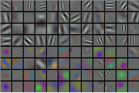
The first modern CNN (Krizhevsky et al. 2012) is largely an evolutionary improvement over LeNet, and it is named AlexNet after one of its inventors, Alex Krizhevsky. It won the 2012 ImageNet challenge and vindicated the bet on learning: in its lowest layers, the network learned feature extractors that resembled the traditional filters, as Figure 7.1.1 shows. Higher layers build upon these representations to capture larger structures, like eyes, noses, and blades of grass, and yet higher layers whole objects, like people, airplanes, and dogs. Ultimately, the final hidden state is a compact representation of the image in which the different categories are easily separated.
AlexNet (2012) and its precursor LeNet (1995) share many architectural elements, which raises the question of why it took so long. The decisive difference is that, over the intervening two decades, the amount of data and the computing power available had each grown by orders of magnitude.
7.1.1.1 Missing Ingredient: Data
Deep models with many layers require large amounts of data in order to enter the regime where they significantly outperform traditional methods based on convex optimization. However, given the limited storage, the expense of imaging sensors, and the tighter research budgets of the 1990s, most research relied on tiny datasets of hundreds or a few thousand low-resolution images, such as those in the UCI collection.
The ImageNet dataset, released in 2009 (Deng et al. 2009), changed this. The 2012 classification challenge supplied roughly 1.2 million training images across 1000 categories drawn from WordNet (Miller 1995), prefiltered by web image search and verified by Amazon Mechanical Turk workers. Class sizes varied, and the source images had varying resolutions; models commonly trained on \(224 \times 224\) crops. The scale exceeded earlier labeled datasets by over an order of magnitude, while the source images retained far more detail than the \(32 \times 32\) thumbnails of the 80-million-image TinyImages dataset (Torralba et al. 2008), so higher-level features could form. The associated ImageNet Large Scale Visual Recognition Challenge (Russakovsky et al. 2015) pushed computer vision and machine learning research to a scale that academics had not previously considered.
7.1.1.2 Missing Ingredient: Hardware
Deep learning models are also voracious consumers of compute cycles: training can take hundreds of epochs, and each iteration passes data through many layers of expensive linear algebra operations. Graphics processing units (GPUs) changed the economics. These chips had been developed to accelerate computer graphics, in particular high-throughput \(4 \times 4\) matrix–vector products, which is math very similar to that of convolutional layers. Around that time NVIDIA and ATI had begun optimizing them for general computing (Fernando 2004) and marketing them as general-purpose GPUs (GPGPUs). Where a CPU core runs at a high clock frequency and spends most of its chip area on the machinery of general control flow (branch predictors, deep pipelines, speculative execution, large caches), a GPU packs thousands of much simpler cores onto one chip. This improves power efficiency because consumption grows roughly quadratically with clock frequency: for the budget of one CPU core running at four times the speed, 16 GPU cores at \(\frac{1}{4}\) the speed deliver \(16 \times \frac{1}{4} = 4\) times the throughput. GPUs also have far wider memory buses, which matters because many deep learning operations are limited by memory bandwidth. A convolution applies the same small program at many output locations and channels, providing exactly this kind of independent work. The effect compounded quickly. In 1999 NVIDIA’s GeForce 256 processed roughly 480 million floating-point operations per second, with no programming framework beyond graphics APIs; by 2012 consumer GPU throughput had grown by roughly three orders of magnitude, and general-purpose GPU interfaces made it accessible without expressing the computation as a graphics pipeline.
This was the situation in 2012 when Alex Krizhevsky and Ilya Sutskever implemented a deep CNN that could run on GPUs. They realized that the computational bottlenecks in CNNs, convolutions and matrix multiplications, are precisely the operations that GPUs parallelize well. Using two NVIDIA GTX 580s with 3 GB of memory each, they implemented fast convolutions. The cuda-convnet code was good enough that for several years it was the industry standard and powered the first couple of years of the deep learning boom.
7.1.2 AlexNet
AlexNet, which employed an 8-layer CNN, won the ImageNet Large Scale Visual Recognition Challenge 2012 by a large margin (Russakovsky et al. 2013). This network showed, for the first time, that the features obtained by learning can transcend manually designed features, breaking the previous paradigm in computer vision.
The architectures of AlexNet and LeNet are closely related, as Figure 7.1.2 illustrates. Note that we provide a slightly streamlined version of AlexNet removing some of the design quirks that were needed in 2012 to make the model fit on two small GPUs.
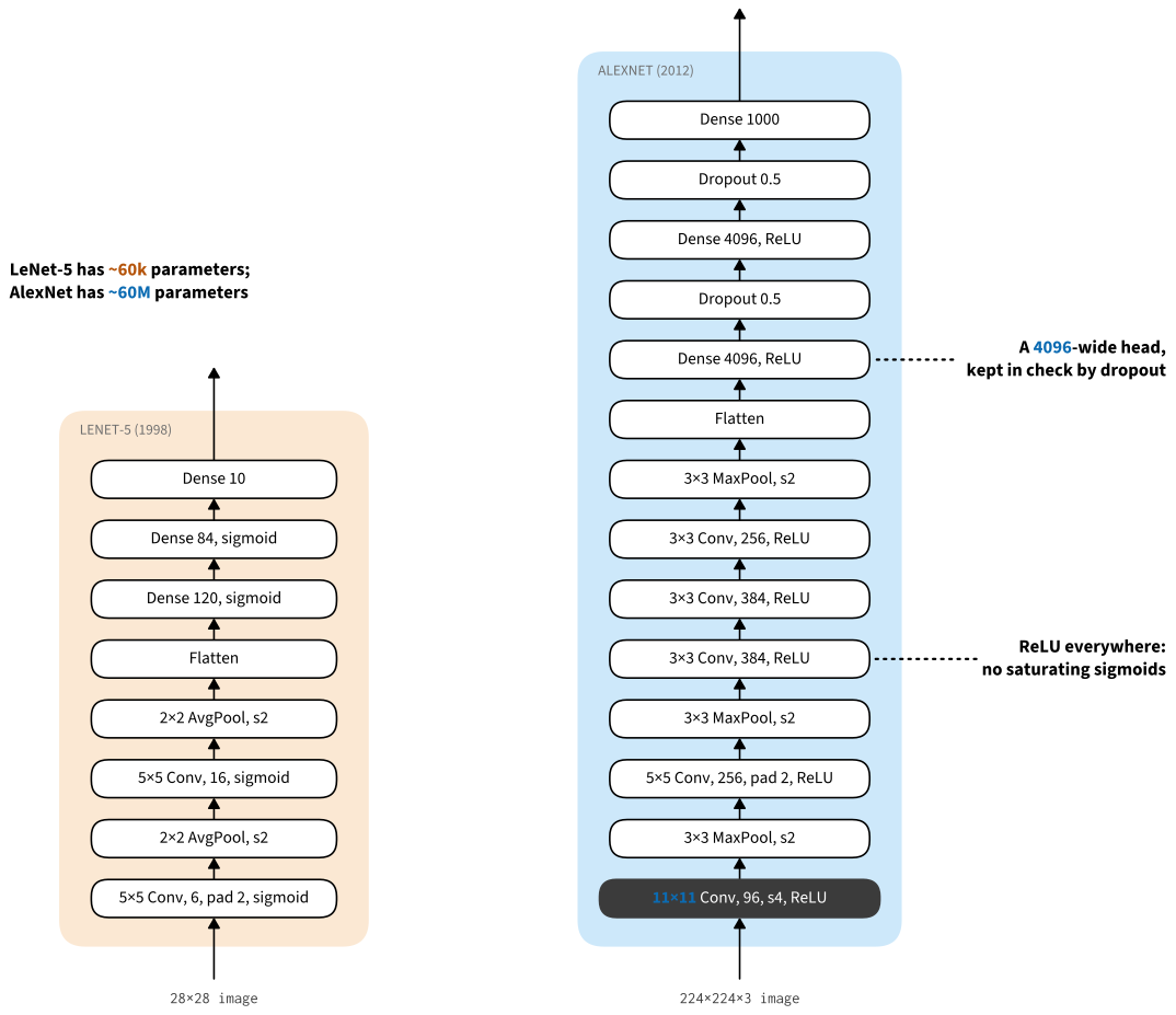
There are also key differences. First, AlexNet is much deeper than the comparatively small LeNet-5. AlexNet consists of eight layers: five convolutional layers, two fully connected hidden layers, and one fully connected output layer. Second, AlexNet used the ReLU instead of the sigmoid as its activation function. We next examine the architecture.
7.1.2.1 Architecture
In AlexNet’s first layer, the convolution window shape is \(11\times11\). Since the images in ImageNet are eight times taller and wider than the MNIST images, objects in ImageNet data tend to occupy more pixels with more visual detail. Consequently, a larger convolution window is needed to capture the object. The convolution window shape in the second layer is reduced to \(5\times5\), followed by \(3\times3\). In addition, after the first, second, and fifth convolutional layers, the network adds max-pooling layers with a window shape of \(3\times3\) and a stride of 2. Moreover, AlexNet has ten times more convolution channels than LeNet.
After the final convolutional layer, there are two huge fully connected layers with 4096 outputs each. Together they account for almost all of the model’s parameters (over 160 MB in single precision). Because of the limited memory in early GPUs, the original AlexNet used a dual data stream design, so that each of their two GPUs could be responsible for storing and computing only its half of the model. GPU memory is rarely that scarce anymore, so our version of the model dispenses with the split.
7.1.2.2 Activation Functions
AlexNet also changed the sigmoid activation function to the simpler ReLU activation function. This makes the computation cheaper, since the ReLU has no exponentiation operation, and, more importantly, it makes training easier: when the output of the sigmoid is very close to 0 or 1, its gradient is almost 0, so poorly initialized parameters may stop receiving updates, whereas the gradient of the ReLU in the positive interval is always 1 (Section 4.1.2).
7.1.2.3 Capacity Control and Preprocessing
AlexNet controls the model complexity of the fully connected layer by dropout (Section 4.6), while LeNet only uses weight decay. To augment the data even further, the training loop of AlexNet added a great deal of image augmentation, such as flipping, clipping, and color changes. This exposes the model to many more variants of each image and thereby reduces overfitting; see Buslaev et al. (2020) for an in-depth review of such preprocessing steps. Augmentation and its descendants have since grown into a central part of how convolutional networks are trained, and we return to them in Section 7.6.
class AlexNet(d2l.Classifier):
    def __init__(self, lr=0.1, num_classes=10):
        super().__init__()
        self.save_hyperparameters()
        self.net = nn.Sequential(
            nn.LazyConv2d(96, kernel_size=11, stride=4),
            nn.ReLU(), nn.MaxPool2d(kernel_size=3, stride=2),
            nn.LazyConv2d(256, kernel_size=5, padding=2), nn.ReLU(),
            nn.MaxPool2d(kernel_size=3, stride=2),
            nn.LazyConv2d(384, kernel_size=3, padding=1), nn.ReLU(),
            nn.LazyConv2d(384, kernel_size=3, padding=1), nn.ReLU(),
            nn.LazyConv2d(256, kernel_size=3, padding=1), nn.ReLU(),
            nn.MaxPool2d(kernel_size=3, stride=2), nn.Flatten(),
            nn.LazyLinear(4096), nn.ReLU(), nn.Dropout(p=0.5),
            nn.LazyLinear(4096), nn.ReLU(),nn.Dropout(p=0.5),
            nn.LazyLinear(num_classes))
        # Note: lazy layers have no parameters at construction time, so weight
        # initialization (d2l.init_cnn) is applied later via apply_init after
        # a dummy forward pass materializes the parameters.
class AlexNet(d2l.Classifier):
def __init__(self, lr=0.1, num_classes=10):
super().__init__()
self.save_hyperparameters()
self.net = tf.keras.models.Sequential([
tf.keras.layers.Conv2D(filters=96, kernel_size=11, strides=4,
activation='relu'),
tf.keras.layers.MaxPool2D(pool_size=3, strides=2),
tf.keras.layers.Conv2D(filters=256, kernel_size=5, padding='same',
activation='relu'),
tf.keras.layers.MaxPool2D(pool_size=3, strides=2),
tf.keras.layers.Conv2D(filters=384, kernel_size=3, padding='same',
activation='relu'),
tf.keras.layers.Conv2D(filters=384, kernel_size=3, padding='same',
activation='relu'),
tf.keras.layers.Conv2D(filters=256, kernel_size=3, padding='same',
activation='relu'),
tf.keras.layers.MaxPool2D(pool_size=3, strides=2),
tf.keras.layers.Flatten(),
tf.keras.layers.Dense(4096, activation='relu'),
tf.keras.layers.Dropout(0.5),
tf.keras.layers.Dense(4096, activation='relu'),
tf.keras.layers.Dropout(0.5),
tf.keras.layers.Dense(num_classes)])class AlexNet(d2l.Classifier):
def __init__(self, lr=0.1, num_classes=10, rngs=None):
super().__init__()
self.save_hyperparameters(ignore=['rngs'])
rngs = (nnx.Rngs(params=d2l.get_key(), dropout=d2l.get_key())
if rngs is None else rngs)
self.net = nnx.Sequential(
nnx.Conv(1, 96, kernel_size=(11, 11), strides=4,
padding='VALID', rngs=rngs),
nnx.relu,
lambda x: nnx.max_pool(x, window_shape=(3, 3), strides=(2, 2)),
nnx.Conv(96, 256, kernel_size=(5, 5), rngs=rngs),
nnx.relu,
lambda x: nnx.max_pool(x, window_shape=(3, 3), strides=(2, 2)),
nnx.Conv(256, 384, kernel_size=(3, 3), rngs=rngs), nnx.relu,
nnx.Conv(384, 384, kernel_size=(3, 3), rngs=rngs), nnx.relu,
nnx.Conv(384, 256, kernel_size=(3, 3), rngs=rngs), nnx.relu,
lambda x: nnx.max_pool(x, window_shape=(3, 3), strides=(2, 2)),
lambda x: x.reshape((x.shape[0], -1)), # flatten
nnx.Linear(5 * 5 * 256, 4096, rngs=rngs),
nnx.relu,
nnx.Dropout(0.5, rngs=rngs),
nnx.Linear(4096, 4096, rngs=rngs),
nnx.relu,
nnx.Dropout(0.5, rngs=rngs),
nnx.Linear(4096, num_classes, rngs=rngs))class AlexNet(d2l.Classifier):
def __init__(self, lr=0.1, num_classes=10):
super().__init__()
self.save_hyperparameters()
self.net = nn.Sequential()
self.net.add(
nn.Conv2D(96, kernel_size=11, strides=4, activation='relu'),
nn.MaxPool2D(pool_size=3, strides=2),
nn.Conv2D(256, kernel_size=5, padding=2, activation='relu'),
nn.MaxPool2D(pool_size=3, strides=2),
nn.Conv2D(384, kernel_size=3, padding=1, activation='relu'),
nn.Conv2D(384, kernel_size=3, padding=1, activation='relu'),
nn.Conv2D(256, kernel_size=3, padding=1, activation='relu'),
nn.MaxPool2D(pool_size=3, strides=2),
nn.Dense(4096, activation='relu'), nn.Dropout(0.5),
nn.Dense(4096, activation='relu'), nn.Dropout(0.5),
nn.Dense(num_classes))
self.net.initialize(init.Xavier())We construct a single-channel data example with both height and width of 224 to observe the output shape of each layer. It matches the AlexNet architecture in Figure 7.1.2.
AlexNet().layer_summary((1, 1, 224, 224))Conv2d output shape: torch.Size([1, 96, 54, 54])
ReLU output shape: torch.Size([1, 96, 54, 54])
MaxPool2d output shape: torch.Size([1, 96, 26, 26])
Conv2d output shape: torch.Size([1, 256, 26, 26])
ReLU output shape: torch.Size([1, 256, 26, 26])
MaxPool2d output shape: torch.Size([1, 256, 12, 12])
Conv2d output shape: torch.Size([1, 384, 12, 12])
ReLU output shape: torch.Size([1, 384, 12, 12])
Conv2d output shape: torch.Size([1, 384, 12, 12])
ReLU output shape: torch.Size([1, 384, 12, 12])
Conv2d output shape: torch.Size([1, 256, 12, 12])
ReLU output shape: torch.Size([1, 256, 12, 12])
MaxPool2d output shape: torch.Size([1, 256, 5, 5])
Flatten output shape: torch.Size([1, 6400])
Linear output shape: torch.Size([1, 4096])
ReLU output shape: torch.Size([1, 4096])
Dropout output shape: torch.Size([1, 4096])
Linear output shape: torch.Size([1, 4096])
ReLU output shape: torch.Size([1, 4096])
Dropout output shape: torch.Size([1, 4096])
Linear output shape: torch.Size([1, 10])AlexNet().layer_summary((1, 224, 224, 1))Conv2D output shape: (1, 54, 54, 96)
MaxPooling2D output shape: (1, 26, 26, 96)
Conv2D output shape: (1, 26, 26, 256)
MaxPooling2D output shape: (1, 12, 12, 256)
Conv2D output shape: (1, 12, 12, 384)
Conv2D output shape: (1, 12, 12, 384)
Conv2D output shape: (1, 12, 12, 256)
MaxPooling2D output shape: (1, 5, 5, 256)
Flatten output shape: (1, 6400)
Dense output shape: (1, 4096)
Dropout output shape: (1, 4096)
Dense output shape: (1, 4096)
Dropout output shape: (1, 4096)
Dense output shape: (1, 10)AlexNet().layer_summary((1, 224, 224, 1))Conv output shape: (1, 54, 54, 96)
custom_jvp output shape: (1, 54, 54, 96)
function output shape: (1, 26, 26, 96)
Conv output shape: (1, 26, 26, 256)
custom_jvp output shape: (1, 26, 26, 256)
function output shape: (1, 12, 12, 256)
Conv output shape: (1, 12, 12, 384)
custom_jvp output shape: (1, 12, 12, 384)
Conv output shape: (1, 12, 12, 384)
custom_jvp output shape: (1, 12, 12, 384)
Conv output shape: (1, 12, 12, 256)
custom_jvp output shape: (1, 12, 12, 256)
function output shape: (1, 5, 5, 256)
function output shape: (1, 6400)
Linear output shape: (1, 4096)
custom_jvp output shape: (1, 4096)
Dropout output shape: (1, 4096)
Linear output shape: (1, 4096)
custom_jvp output shape: (1, 4096)
Dropout output shape: (1, 4096)
Linear output shape: (1, 10)AlexNet().layer_summary((1, 1, 224, 224))Conv2D output shape: (1, 96, 54, 54)
MaxPool2D output shape: (1, 96, 26, 26)
Conv2D output shape: (1, 256, 26, 26)
MaxPool2D output shape: (1, 256, 12, 12)
Conv2D output shape: (1, 384, 12, 12)
Conv2D output shape: (1, 384, 12, 12)
Conv2D output shape: (1, 256, 12, 12)
MaxPool2D output shape: (1, 256, 5, 5)
Dense output shape: (1, 4096)
Dropout output shape: (1, 4096)
Dense output shape: (1, 4096)
Dropout output shape: (1, 4096)
Dense output shape: (1, 10)7.1.3 Training
Although AlexNet was trained on ImageNet in Krizhevsky et al. (2012), we use Fashion-MNIST here since training an ImageNet model to convergence could take hours or days even on a modern GPU. One of the problems with applying AlexNet directly on Fashion-MNIST is that its images have lower resolution (\(28 \times 28\) pixels) than ImageNet images. To make things work, we upsample them to \(224 \times 224\). Upsampling increases computation without adding information. We nevertheless do so here to preserve the AlexNet architecture. We perform this resizing with the resize argument in the d2l.FashionMNIST constructor.
We can now train AlexNet. Compared to LeNet in Section 6.6, the main change here is the use of a smaller learning rate and much slower training due to the deeper and wider network, the higher image resolution, and the more costly convolutions.
model = AlexNet(lr=0.01)
data = d2l.FashionMNIST(batch_size=128, resize=(224, 224))
trainer = d2l.Trainer(max_epochs=10, num_gpus=1)
if tab.selected('pytorch'):
    # Lazy layers have no weights at construction time; apply_init runs a
    # dummy forward pass to materialize parameters and then applies init_cnn.
    model.apply_init([next(iter(data.get_dataloader(True)))[0]], d2l.init_cnn)
trainer.fit(model, data)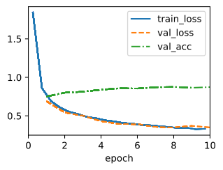
trainer = d2l.Trainer(max_epochs=10)
data = d2l.FashionMNIST(batch_size=128, resize=(224, 224))
with d2l.try_gpu():
    model = AlexNet(lr=0.01)
    trainer.fit(model, data)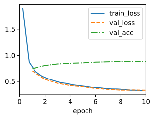
model = AlexNet(lr=0.01)
data = d2l.FashionMNIST(batch_size=128, resize=(224, 224))
trainer = d2l.Trainer(max_epochs=10, num_gpus=1)
if tab.selected('pytorch'):
    # Lazy layers have no weights at construction time; apply_init runs a
    # dummy forward pass to materialize parameters and then applies init_cnn.
    model.apply_init([next(iter(data.get_dataloader(True)))[0]], d2l.init_cnn)
trainer.fit(model, data)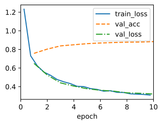
model = AlexNet(lr=0.01)
data = d2l.FashionMNIST(batch_size=128, resize=(224, 224))
trainer = d2l.Trainer(max_epochs=10, num_gpus=1)
if tab.selected('pytorch'):
    # Lazy layers have no weights at construction time; apply_init runs a
    # dummy forward pass to materialize parameters and then applies init_cnn.
    model.apply_init([next(iter(data.get_dataloader(True)))[0]], d2l.init_cnn)
trainer.fit(model, data)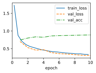
7.1.4 Discussion
AlexNet retains LeNet’s convolutional encoder and dense classification head, but it is substantially wider and deeper. ReLU activations ease optimization, and dropout regularizes the large dense layers. Modern frameworks express the architecture compactly; the original work also required specialized GPU kernels and a distributed training implementation.
The dense head is AlexNet’s main efficiency limitation. Its first two matrices have shapes \(6400 \times 4096\) and \(4096 \times 4096\), together requiring about 164 MiB in 32-bit floating point and tens of millions of multiply-adds per example. Later architectures replace this head with global pooling and a single linear layer. In our Fashion-MNIST run, the plotted training and validation losses remain close. This observation is consistent with adequate regularization for this run, but it does not isolate dropout from the effects of data preprocessing, optimization, or task difficulty.
Although it seems that there are only a few more lines in AlexNet’s implementation than in LeNet’s, it took the academic community many years to embrace this conceptual change and take advantage of its excellent experimental results. This was also due to the lack of efficient computational tools. At the time neither DistBelief (Dean et al. 2012) nor Caffe (Jia et al. 2014) existed, and Theano (Bergstra et al. 2010), the first widely used automatic-differentiation framework, still lacked many features its successors would bring. Implementing a new architecture turned from an engineering project into routine work only as such frameworks matured, from Theano to TensorFlow (Abadi et al. 2016) and later PyTorch (Paszke et al. 2019) and JAX (Frostig et al. 2018).
7.1.5 Exercises
- Following up on the discussion above, analyze the computational properties of AlexNet.
- Compute the memory footprint for convolutions and fully connected layers, respectively. Which one dominates?
- Calculate the computational cost for the convolutions and the fully connected layers.
- How does the memory (read and write bandwidth, latency, size) affect computation? Is there any difference in its effects for training and inference?
- You are a chip designer and need to trade off computation and memory bandwidth. For example, a faster chip requires more power and possibly a larger chip area. More memory bandwidth requires more pins and control logic, thus also more area. How do you optimize?
- Why do engineers no longer report performance benchmarks on AlexNet?
- Try increasing the number of epochs when training AlexNet. Compared with LeNet, how do the results differ? Why?
- AlexNet may be too complex for the Fashion-MNIST dataset, in particular due to the low resolution of the initial images.
- Try simplifying the model to make the training faster, while ensuring that the accuracy does not drop significantly.
- Design a better model that works directly on \(28 \times 28\) images.
- Modify the batch size, and observe the changes in throughput (images/s), accuracy, and GPU memory.
- Apply dropout and ReLU to LeNet-5. Does it improve? Can you improve things further by preprocessing to take advantage of the invariances inherent in the images?
- Can you make AlexNet overfit? Which feature do you need to remove or change to break training?