%matplotlib inline
from d2l import torch as d2l
import gymnasium as gym
import numpy as np
import torch
from torch import nn
torch.set_num_threads(1)15.1 Actor-Critic Methods and Multi-Step Returns
Section 14.7 estimated advantages from complete sampled returns, so an update could be formed only after an episode ended. An actor–critic method instead uses a learned value function to bootstrap from incomplete trajectories (Barto et al. 1983; Konda and Tsitsiklis 2000). The actor is the policy \(\pi_\theta\), and the critic estimates its value \(V^{\pi_\theta}\).
Bootstrapping reduces the amount of future randomness in each target but introduces error from the critic. This section derives the one-step temporal-difference target, extends it to \(n\)-step and \(\lambda\)-returns, and implements generalized advantage estimation (GAE). Experiments on CartPole compare these estimators through their gradient error, training stability, and sensitivity to critic fitting.
%matplotlib inline
from d2l import jax as d2l
from flax import nnx
import gymnasium as gym
import jax
from jax import numpy as jnp
import numpy as np
import optax
We retain the CartPole environment, discount \(0.99\), and one-hidden-layer ActorCritic.mlp model from Section 14.7. The new hyperparameter critic_steps specifies the number of critic regression passes per batch. Unless stated otherwise, we use twenty passes and recompute the target before each pass.
gamma, num_updates, batch_episodes = 0.99, 100, 8
num_seeds, critic_steps, grad_clip = 3, 20, 0.5
if tab.selected('pytorch'):
    def cartpole_agent(seed):
        torch.manual_seed(seed)
        return d2l.ActorCritic.mlp(4, 2)
if tab.selected('jax'):
    def cartpole_agent(seed):
        return d2l.ActorCritic.mlp(4, 2, rngs=nnx.Rngs(seed))
gamma, num_updates, batch_episodes = 0.99, 100, 8
num_seeds, critic_steps, grad_clip = 3, 20, 0.5
if tab.selected('pytorch'):
def cartpole_agent(seed):
torch.manual_seed(seed)
return d2l.ActorCritic.mlp(4, 2)
if tab.selected('jax'):
def cartpole_agent(seed):
return d2l.ActorCritic.mlp(4, 2, rngs=nnx.Rngs(seed))15.1.1 Bootstrapping the Reward-to-Go
15.1.1.1 The TD Error
Write out one step of what the reward-to-go contains,
\[\hat{G}_t = r_t + \gamma\, \hat{G}_{t+1}, \tag{15.1.1}\]
and recall what the learned baseline of Section 14.6 is trained on: \(\hat{V}(s_{t+1})\) regresses toward exactly the quantity that \(\hat{G}_{t+1}\) samples. So stop waiting for the sample and substitute the prediction, \(\hat{G}_t \approx r_t + \gamma \hat{V}(s_{t+1})\). The weight on the score at step \(t\) was \(\hat{G}_t - \hat{V}(s_t)\); after the substitution it becomes
\[\delta_t = r_t + \gamma\, \hat{V}(s_{t+1}) - \hat{V}(s_t), \tag{15.1.2}\]
with the convention \(\hat{V}(s_{t+1}) = 0\) when \(s_{t+1}\) is terminal. This is the temporal-difference error of Equation 14.4.4, adapted to policy evaluation. Q-learning bootstraps on the greedy continuation \(\max_{a'} \hat{Q}(s', a')\) because it estimates \(Q^*\); here the bootstrap uses the current policy’s continuation value \(\hat{V}(s_{t+1})\). As in Q-learning, the terminal mask is determined by terminated, not truncated, because a time limit stops the observation without making the continuation value zero (Section 14.1). The bootstrap function below returns a numpy array, so the target contains no autograd history and requires no explicit detach.
@d2l.add_to_class(d2l.Batch)
def td_target(self, bootstrap, gamma):
    """r_t + gamma (1 - terminated) V(s'), by a numpy bootstrap."""
return self.rew + gamma * (1 - self.term) * bootstrap(self.next_obs)@d2l.add_to_class(d2l.Batch)
def td_target(self, bootstrap, gamma):
"""r_t + gamma (1 - terminated) V(s'), by a numpy bootstrap."""
return self.rew + gamma * (1 - self.term) * bootstrap(self.next_obs)As in Equation 14.6.4, we omit the factor \(\gamma^t\) from the actor update. The consequences of this convention were discussed in Section 14.6.
15.1.1.2 The TD Error as an Advantage Estimate
The TD error is not merely cheaper than the Monte Carlo weight; it estimates the same thing. Suppose for a moment the critic were exact, \(\hat{V} = V^\pi\). Averaging Equation 15.1.2 over the next state,
\[E\big[ \delta_t \mid s_t, a_t \big] = r(s_t, a_t) + \gamma \sum_{s'} P(s' \mid s_t, a_t)\, V^{\pi}(s') - V^{\pi}(s_t) = Q^{\pi}(s_t, a_t) - V^{\pi}(s_t),\]
where the second equality is Equation 14.2.7 written with \(V^\pi\). The right-hand side is the advantage Equation 14.2.4 of the action taken, the exact quantity the learned baseline of Section 14.6 estimated with \(\hat{G}_t - \hat{V}(s_t)\). So a single transition, one reward plus two critic evaluations, yields an unbiased one-sample estimate of the advantage, where the Monte Carlo estimate needed the entire remaining trajectory.
During training \(\hat{V}\) is generally not equal to \(V^\pi\). Consequently, \(\delta_t\) is a biased estimate of the advantage, and the resulting policy update is not an unbiased gradient estimator of \(J(\theta)\). The baseline lemma of Section 14.6 does not apply to the bootstrap term: unlike a state-dependent baseline at time \(t\), \(\hat{V}(s_{t+1})\) depends on the sampled action through the next state. Exercise 1 identifies the corresponding step in the proof. Bootstrapping therefore exchanges some variance for bias.
15.1.1.3 The Critic as Sampled Policy Evaluation
The critic update is a sampled form of policy evaluation. In Section 14.2, policy evaluation applied a Bellman expectation operator whose fixed point is \(V^\pi\). Regressing \(\hat{V}(s_t)\) toward \(r_t + \gamma \hat{V}(s_{t+1})\) replaces that expectation by one sampled transition, just as Q-learning replaced the Bellman optimality expectation by a sample in Section 14.4. Actor-critic can therefore be viewed as approximate generalized policy iteration: the critic estimates \(V^{\pi_\theta}\), while the actor improves the policy using that estimate. Because the regression target itself contains \(\hat{V}\), the critic update is a semi-gradient toward a fixed point rather than gradient descent on a fixed supervised-learning objective.
15.1.1.4 The Bias-Variance Trade-off
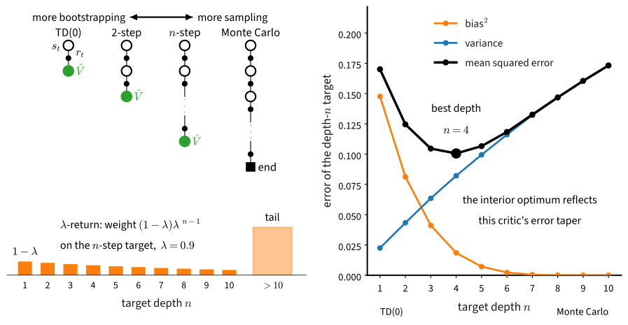
The two advantage estimates have complementary errors. The Monte Carlo estimate is unbiased but includes randomness from every remaining transition, so its variance tends to grow with the horizon. The one-step TD error depends on only one transition, but it inherits bias from the critic. Targets that bootstrap after \(n\) steps interpolate between these cases. In the synthetic chain in Figure 15.1.1, the critic becomes more accurate near termination; increasing \(n\) therefore reduces bias and increases variance, with the smallest mean squared error at an intermediate depth. This pattern depends on the example and is not a general monotonicity result.
15.1.2 The Actor-Critic Algorithm
15.1.2.1 The Actor and Critic Updates
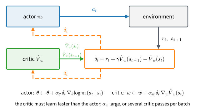
Both learners now update from the same scalar. Writing \(\hat{V}_w\) for the critic’s parameters, the updates after the transition \((s_t, a_t, r_t, s_{t+1})\) are
\[w \leftarrow w + \alpha_w\, \delta_t\, \nabla_w \hat{V}_w(s_t), \qquad \theta \leftarrow \theta + \alpha_\theta\, \delta_t\, \nabla_\theta \log \pi_\theta(a_t \mid s_t). \tag{15.1.3}\]
The critic’s update is the sampled policy evaluation of the previous section, a semi-gradient step toward the one-step target; the actor’s is the policy gradient of Section 14.6 with \(\delta_t\) as the advantage weight. One number does both jobs: \(\delta_t\) tells the critic how wrong its prediction was, and it tells the actor whether the action just taken was better or worse than the state’s average. And because \(\delta_t\) needs only a single transition, Equation 15.1.3 can be applied at every step as the agent acts, the way Q-learning updates its table; nothing must terminate before learning starts, so the method extends to tasks that never end. REINFORCE, with or without a baseline, cannot say the same.
15.1.2.2 Two Timescales
The actor and critic have different optimization problems. Actor updates change the policy and hence the value function being estimated; critic updates also change the bootstrapped targets. If the actor changes much faster than the critic, its advantages may be evaluated with stale value estimates. Classical two-timescale results address this interaction using separated, decaying step-size schedules under assumptions that this experiment does not meet. Here both heads use the same nominal learning rate, with critic_steps regression passes per batch. This is a heuristic, not an implementation of the theorem’s schedule.
15.1.2.3 A Batched Actor-Critic and A2C
What we implement below is not the fully online Equation 15.1.3, and the difference deserves a careful name. The code collects a batch of eight episodes from one environment, gives the critic its critic_steps regression passes on the batch’s one-step targets, and then takes a single actor step weighted by the TD errors of the freshly updated critic: call it a batched on-policy actor-critic. Its production relative is A2C, the advantage actor-critic, which conventionally denotes the synchronous multi-actor form: many environments stepped in lockstep with \(n\)-step rollouts, itself the synchronous descendant of an asynchronous original (Mnih et al. 2016). Our single-environment, whole-episode loop keeps A2C’s estimator and drops its vectorization. Exercise 5 takes up the fully online form, one update per transition with no batch at all, and what goes wrong there is a preview of Section 15.4.
We first modify d2l.policy_step to cap the actor’s gradient norm at the commonly used value \(0.5\). The function also reports the norm before clipping so that the experiments below can compare the scale of different advantage estimators.
def policy_step_clip(ac, batch, w, clip=grad_clip):
    """d2l.policy_step with the actor's gradient norm capped at `clip`;
    returns the norm measured before the cap."""
    obs, act = torch.as_tensor(batch.obs), torch.as_tensor(batch.act)
    loss = -(torch.as_tensor(w) * ac.log_prob(obs, act)).mean()
    ac.opt_pi.zero_grad()
    loss.backward()
    gnorm = nn.utils.clip_grad_norm_(ac.policy.parameters(), clip)
    ac.opt_pi.step()
    return float(gnorm)
def policy_step_clip(ac, batch, w, clip=grad_clip):
"""d2l.policy_step with the actor's gradient norm capped at `clip`;
returns the norm measured before the cap. `_pad` and `_actor_pass`,
defined with the critic's compilation story two cells below, are
resolved at the first call."""
size = 1 << max(6, (len(w) - 1).bit_length())
gnorm = _actor_pass(ac.policy, ac.opt_pi, _pad(batch.obs, size),
_pad(batch.act, size), _pad(w, size),
jnp.float32(len(w)), jnp.float32(clip))
return float(gnorm)The second piece is per-framework speed, not algorithm, and follows the compilation rule of Section 13.3: compile what has a fixed shape and runs hot, leave ragged shapes eager. The acting forward runs a few hundred thousand times at one fixed shape, so the jax tab compiles and caches it exactly as Section 14.7 did; the pytorch tab’s eager dispatch is already cheap at this scale and needs nothing.
_act_probs = nnx.jit(lambda net, obs: jax.nn.softmax(net(obs), -1))

def _probs(ac, obs):   # the fixed-shape acting forward, compiled and
    if not hasattr(ac, '_fwd'):        # cached as in :numref:`sec_deeprl`
        ac._fwd = nnx.cached_partial(_act_probs, ac.policy)
    return np.asarray(ac._fwd(jnp.asarray(obs)))

@d2l.add_to_class(d2l.ActorCritic)
def act(self, obs, rng):
    p = _probs(self, obs)
    return int(rng.choice(len(p), p=p))

@d2l.add_to_class(d2l.ActorCritic)
def act_greedy(self, obs, rng=None):
    return int(_probs(self, obs).argmax())
The critic’s regression and the actor’s clipped step are this section’s hot loops, together tens of thousands of passes per run, each on a batch of a few fixed lengths. Padding every batch to a power-of-two length makes the shape one of a handful and lets the jitted passes and the jitted value read that computes the critic’s target compile once per bucket rather than once per batch; a mask, or zero-padded weights, keeps the padded entries out of each loss.
# Eager per-pass cost is about a millisecond in this tab; the library
# helper needs no compilation story here, unlike its jax sibling.
fit_value = d2l.fit_value
def _pad(x, size):
return jnp.asarray(np.pad(x, ((0, size - len(x)),) + ((0, 0),)
* (x.ndim - 1)))
_value_fwd = nnx.jit(lambda net, obs: net(obs).squeeze(-1))
@d2l.add_to_class(d2l.ActorCritic)
def value_np(self, obs): # batched reads only, padded to the bucket size
size = 1 << max(6, (len(obs) - 1).bit_length())
return np.asarray(_value_fwd(self.value, _pad(obs, size)))[:len(obs)]
@nnx.jit
def _critic_pass(value, opt, obs, target, mask):
loss, grads = nnx.value_and_grad(lambda v: (mask * (
v(obs).squeeze(-1) - target) ** 2).sum() / mask.sum())(value)
opt.update(value, grads)
return loss
@nnx.jit
def _actor_pass(policy, opt, obs, act, adv, n_real, clip):
def loss_fn(p): # zero-padded adv silences the padded rows exactly
logp = jax.nn.log_softmax(p(obs), -1)[jnp.arange(obs.shape[0]), act]
return -(adv * logp).sum() / n_real
grads = nnx.grad(loss_fn)(policy)
gnorm = optax.global_norm(grads)
grads = jax.tree.map(lambda g: g * jnp.minimum(1.0, clip / gnorm), grads)
opt.update(policy, grads)
return gnorm
def fit_value(ac, obs, target, num_steps=1):
"""d2l.fit_value, padded to a power-of-two length: the jitted pass
compiles once per size bucket (:numref:`sec_compilation`)."""
size = 1 << max(6, (len(target) - 1).bit_length())
mask = jnp.asarray((np.arange(size) < len(target)).astype(np.float32))
for _ in range(num_steps):
loss = _critic_pass(ac.value, ac.opt_v, _pad(obs, size),
_pad(target, size), mask)
return float(loss)Now the two training functions, side by side. The Monte Carlo reference is train_reinforce of Section 14.7 with two mechanical changes: the agent arrives from the caller, following the pattern of Section 14.4’s caller-owned tables, so that the last cell of this section can audit the trained agents; and the actor’s step goes through the clipped variant and yields its gradient norm, a diagnostic returned as data.
def train_reinforce(seed, ac, num_updates=num_updates):
    """sec_deeprl's learned-baseline REINFORCE; the agent is caller-owned
    and the actor step reports its pre-clip gradient norm."""
    rng, env = np.random.default_rng(seed), gym.make('CartPole-v1')
    env.reset(seed=seed)
    for _ in range(num_updates):
        batch = d2l.rollout(env, ac.act, batch_episodes, rng)
        G = batch.reward_to_go(gamma)
        w = d2l.normalize(G - ac.value_np(batch.obs))
        gnorm = policy_step_clip(ac, batch, w)
        fit_value(ac, batch.obs, G)
        yield float(batch.episode_returns().mean()), gnorm
def train_reinforce(seed, ac, num_updates=num_updates):
"""sec_deeprl's learned-baseline REINFORCE; the agent is caller-owned
and the actor step reports its pre-clip gradient norm."""
rng, env = np.random.default_rng(seed), gym.make('CartPole-v1')
env.reset(seed=seed)
for _ in range(num_updates):
batch = d2l.rollout(env, ac.act, batch_episodes, rng)
G = batch.reward_to_go(gamma)
w = d2l.normalize(G - ac.value_np(batch.obs))
gnorm = policy_step_clip(ac, batch, w)
fit_value(ac, batch.obs, G)
yield float(batch.episode_returns().mean()), gnormActor–critic modifies the final part of the preceding training loop. The critic regresses on the one-step bootstrapped target rather than reward-to-go and takes critic_steps passes before the actor update. Each pass recomputes the target from the current critic, so this is fitted TD with a moving target rather than fixed-target regression. Section 15.4 will instead freeze a separate target network when learning off-policy. The actor uses the TD error from Equation 15.1.2, normalized within the batch, as its weight.
def train_ac(seed, ac, num_updates=num_updates):
    """The same loop with the sampled tail replaced by the bootstrap."""
    rng, env = np.random.default_rng(seed), gym.make('CartPole-v1')
    env.reset(seed=seed)
    for _ in range(num_updates):
        batch = d2l.rollout(env, ac.act, batch_episodes, rng)
        for _ in range(critic_steps):   # fresh target, one pass, repeat
            fit_value(ac, batch.obs, batch.td_target(ac.value_np, gamma))
        delta = batch.td_target(ac.value_np, gamma) - ac.value_np(batch.obs)
        gnorm = policy_step_clip(ac, batch, d2l.normalize(delta))
        yield float(batch.episode_returns().mean()), gnorm
def train_ac(seed, ac, num_updates=num_updates):
"""The same loop with the sampled tail replaced by the bootstrap."""
rng, env = np.random.default_rng(seed), gym.make('CartPole-v1')
env.reset(seed=seed)
for _ in range(num_updates):
batch = d2l.rollout(env, ac.act, batch_episodes, rng)
for _ in range(critic_steps): # fresh target, one pass, repeat
fit_value(ac, batch.obs, batch.td_target(ac.value_np, gamma))
delta = batch.td_target(ac.value_np, gamma) - ac.value_np(batch.obs)
gnorm = policy_step_clip(ac, batch, d2l.normalize(delta))
yield float(batch.episode_returns().mean()), gnormThree seeds each, with the agents kept. The reference arm first:
agents = {name: [cartpole_agent(s) for s in range(num_seeds)]
          for name in ('REINFORCE + baseline', 'actor-critic')}
runs = {'REINFORCE + baseline': np.array(
    [list(train_reinforce(s, agents['REINFORCE + baseline'][s]))
     for s in range(num_seeds)])}
agents = {name: [cartpole_agent(s) for s in range(num_seeds)]
for name in ('REINFORCE + baseline', 'actor-critic')}
runs = {'REINFORCE + baseline': np.array(
[list(train_reinforce(s, agents['REINFORCE + baseline'][s]))
for s in range(num_seeds)])}Then the bootstrapped arm, and the comparison:
runs['actor-critic'] = np.array(
    [list(train_ac(s, agents['actor-critic'][s]))
     for s in range(num_seeds)])
d2l.plot_curves({name: r[:, :, 0] for name, r in runs.items()},
                xlabel='update', ylabel='mean return of the batch',
                reference=500)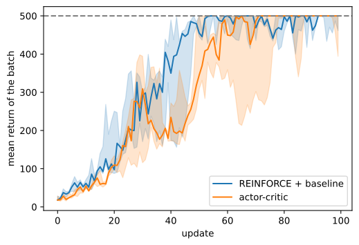
runs['actor-critic'] = np.array(
    [list(train_ac(s, agents['actor-critic'][s]))
     for s in range(num_seeds)])
d2l.plot_curves({name: r[:, :, 0] for name, r in runs.items()},
                xlabel='update', ylabel='mean return of the batch',
                reference=500)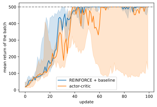
The two curves are the trade of Figure 15.1.1 drawn by the algorithms themselves. Actor-critic starts slower: for its first stretch the critic is still wrong, the TD errors point in poorly chosen directions, and the biased updates buy little, while the Monte Carlo weight is correct on average from the first batch. Then the curves stop differing in level, both reach the neighborhood of the ceiling, and start differing in texture. A batch mean of \(500\) means every one of the batch’s eight episodes ran the full 500 steps, a perfect batch; \(500\) is CartPole’s structural ceiling, so it can be tied but never beaten, and the informative comparison is not who is higher but who, having arrived, stays. The claim is checkable in four lines:
def longest_streak(hits):
    """The longest run of consecutive True entries."""
    best = run = 0
    for h in hits:
        run = run + 1 if h else 0
        best = max(best, run)
    return best

for name, r in runs.items():
    print(f'{name:>20}: longest stretch of perfect batches, per seed: '
          f'{[longest_streak(row == 500) for row in r[:, :, 0]]}')
REINFORCE + baseline: longest stretch of perfect batches, per seed: [6, 7, 4]
actor-critic: longest stretch of perfect batches, per seed: [36, 26, 11]def longest_streak(hits):
"""The longest run of consecutive True entries."""
best = run = 0
for h in hits:
run = run + 1 if h else 0
best = max(best, run)
return best
for name, r in runs.items():
print(f'{name:>20}: longest stretch of perfect batches, per seed: '
f'{[longest_streak(row == 500) for row in r[:, :, 0]]}')REINFORCE + baseline: longest stretch of perfect batches, per seed: [26, 13, 22]
actor-critic: longest stretch of perfect batches, per seed: [39, 22, 3]Both methods reach the maximum batch return, but the bootstrapped runs remain there for longer consecutive intervals in every framework. The streak length is only a visualization of these runs: it depends on policy quality, batch size, environment randomness, and estimator variance, so it is not a standard stability metric.
The difference is consistent with the estimators’ variance. A Monte Carlo weight contains the random outcomes of the entire remaining trajectory, so even a good policy can produce a lower-return update batch. A one-step temporal-difference weight replaces that tail with a critic estimate. The critic introduces bias early in training but reduces the variance that causes later fluctuations.
The training functions also brought back a second number, and it justifies the clip. Both methods scale their weights to unit variance before the update, so it is tempting to assume both take steps of the same size:
for name, r in runs.items():
    g = r[:, :, 1].ravel()
    print(f'{name:>20}: median pre-clip gradient norm {np.median(g):5.2f}, '
          f'clip binds on {(g > grad_clip).mean():4.0%} of updates')
REINFORCE + baseline: median pre-clip gradient norm 0.04, clip binds on 0% of updates
actor-critic: median pre-clip gradient norm 0.40, clip binds on 35% of updatesfor name, r in runs.items():
g = r[:, :, 1].ravel()
print(f'{name:>20}: median pre-clip gradient norm {np.median(g):5.2f}, '
f'clip binds on {(g > grad_clip).mean():4.0%} of updates')REINFORCE + baseline: median pre-clip gradient norm 0.03, clip binds on 0% of updates
actor-critic: median pre-clip gradient norm 0.33, clip binds on 30% of updatesIn these runs, actor–critic gradients are roughly an order of magnitude larger. The norm clip activates on about one third of actor–critic updates and on none of the Monte Carlo updates. The baseline identity from Section 14.6 helps explain this difference: state-dependent variance contributes nothing to the expected policy gradient, and the Monte Carlo weight contains more of it, whereas the temporal-difference error is more strongly action-dependent. Gradient norm alone does not measure signal quality, but the result shows that the two estimators can produce different update scales at the same learning rate. Section 15.2 develops methods for controlling such policy updates.
15.1.2.4 The Critic’s Moving Target and Data Freshness
Every batch in this experiment comes from the current policy and from the states that policy visits. A critic error that affects current behavior is therefore likely to receive relevant transitions in the next batch, reducing the distributional mismatch between critic training and use. This feedback resembles the self-correction described in Section 14.4.
Fresh data do not guarantee stability. Nonlinear temporal-difference regression can diverge on-policy, and classical convergence results assume linear critics and two-timescale step sizes that this implementation does not use (Tsitsiklis and Van Roy 1997). In this experiment, the reduced mismatch is sufficient for stable training. To compare the two estimators directly, we rerun train_ac and measure the temporal-difference error and Monte Carlo advantage on each shared batch.
rng, env = np.random.default_rng(0), gym.make('CartPole-v1')
ac = cartpole_agent(0)
env.reset(seed=0)
trace = []
for _ in range(num_updates):
    b = d2l.rollout(env, ac.act, batch_episodes, rng)
    for _ in range(critic_steps):
        fit_value(ac, b.obs, b.td_target(ac.value_np, gamma))
    V = ac.value_np(b.obs)
    delta = b.td_target(ac.value_np, gamma) - V
    A_mc = b.reward_to_go(gamma) - V
    trace.append((np.corrcoef(delta, A_mc)[0, 1], delta.var(), A_mc.var()))
    policy_step_clip(ac, b, d2l.normalize(delta))
trace = np.array(trace)
print(f'corr(TD error, MC advantage): mean {trace[:10, 0].mean():.2f} over '
      f'the first ten updates, {trace[-50:, 0].mean():.2f} over the last 50')
d2l.plot_curves({'corr(TD error, MC advantage)': trace[:, 0]},
                xlabel='update', ylabel='correlation', smooth=10)
corr(TD error, MC advantage): mean 0.30 over the first ten updates, 0.01 over the last 50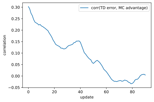
rng, env = np.random.default_rng(0), gym.make('CartPole-v1')
ac = cartpole_agent(0)
env.reset(seed=0)
trace = []
for _ in range(num_updates):
    b = d2l.rollout(env, ac.act, batch_episodes, rng)
    for _ in range(critic_steps):
        fit_value(ac, b.obs, b.td_target(ac.value_np, gamma))
    V = ac.value_np(b.obs)
    delta = b.td_target(ac.value_np, gamma) - V
    A_mc = b.reward_to_go(gamma) - V
    trace.append((np.corrcoef(delta, A_mc)[0, 1], delta.var(), A_mc.var()))
    policy_step_clip(ac, b, d2l.normalize(delta))
trace = np.array(trace)
print(f'corr(TD error, MC advantage): mean {trace[:10, 0].mean():.2f} over '
      f'the first ten updates, {trace[-50:, 0].mean():.2f} over the last 50')
d2l.plot_curves({'corr(TD error, MC advantage)': trace[:, 0]},
                xlabel='update', ylabel='correlation', smooth=10)
corr(TD error, MC advantage): mean 0.33 over the first ten updates, -0.03 over the last 50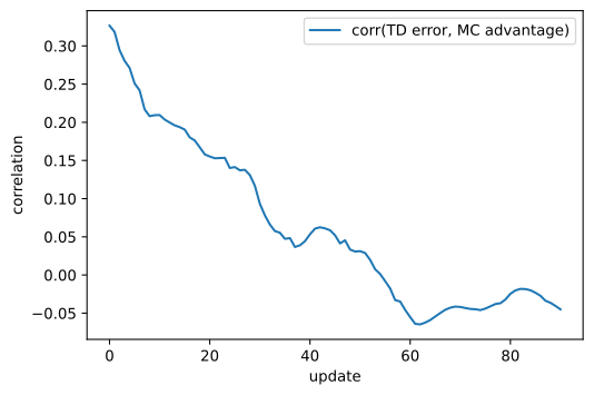
When episodes last a few dozen steps, the two weights have correlation near \(0.3\); after episodes extend to hundreds of steps, the measured correlation approaches zero. Expanding Equation 15.1.2 gives \(\hat{G}_t-\hat{V}(s_t)=\delta_t+\gamma(\hat{G}_{t+1}-\hat{V}(s_{t+1}))\). The Monte Carlo advantage therefore contains the one-step temporal-difference error plus the discounted remainder of the trajectory. As the horizon grows, this additional tail contributes increasing variance.
The correlation is a descriptive diagnostic, not a certificate that the critic is accurate. It also changes with the policy, the state distribution, and the scales of both estimators. A direct critic evaluation would instead freeze the policy and compare predicted values with a reference. Here we next compare the absolute variances of the two policy weights:
print(f'median variance, MC advantage over TD error: '
      f'{np.median(trace[:, 2] / trace[:, 1]):.0f}x')
d2l.plot_curves({'TD error': trace[:, 1], 'MC advantage': trace[:, 2]},
                xlabel='update', ylabel='variance of the weight', smooth=10)
median variance, MC advantage over TD error: 114x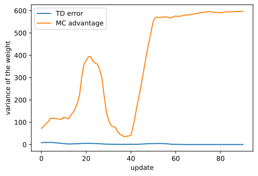
print(f'median variance, MC advantage over TD error: '
      f'{np.median(trace[:, 2] / trace[:, 1]):.0f}x')
d2l.plot_curves({'TD error': trace[:, 1], 'MC advantage': trace[:, 2]},
                xlabel='update', ylabel='variance of the weight', smooth=10)
median variance, MC advantage over TD error: 318x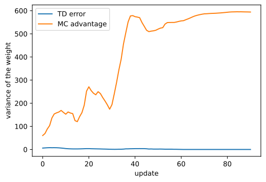
As episodes approach 500 steps, the variance of the Monte Carlo weight grows from tens to several hundred squared units. The temporal-difference error depends on one reward and one transition, so its variance remains much smaller and decreases further as the critic improves. The median variance ratio exceeds one hundred. Averaging eight trajectories per update reduces the Monte Carlo variance enough for REINFORCE to train, but does not remove its dependence on the horizon.
Here the critic is trained on fresh on-policy data, and its target is recomputed after each update. When a value function is instead trained on replayed off-policy data while retaining a bootstrap target, the same semi-gradient update can diverge. Section 15.4 addresses this problem by evaluating the bootstrap with a second network whose parameters are held fixed for several updates. This target network reduces the rate at which the regression target moves.
15.1.3 n-Step Returns, Lambda-Returns and GAE
15.1.3.1 n-Step Returns
The one-step target and the Monte Carlo return are endpoints of a family. Include \(n\) sampled rewards and then bootstrap from the critic:
\[\hat{G}^{(n)}_t = r_t + \gamma\, r_{t+1} + \cdots + \gamma^{n-1} r_{t+n-1} + \gamma^n\, \hat{V}(s_{t+n}), \tag{15.1.4}\]
and use \(\hat{G}^{(n)}_t-\hat{V}(s_t)\) as the advantage estimate. For \(n=1\), this is \(\delta_t\); when \(n\) extends to the end of the episode, it becomes the Monte Carlo advantage. Increasing \(n\) discounts the critic’s error by \(\gamma^n\) and evaluates it at a later state, but also adds another sampled reward and transition. The result is the bias–variance trade-off measured in Figure 15.1.1.
15.1.3.2 The Lambda-Return and the Telescoping Identity
Rather than pick one depth, average them all, with geometric weights that make the average computable:
\[\hat{A}^{\textrm{GAE}}_t = (1 - \lambda) \sum_{n=1}^{\infty} \lambda^{n-1} \big( \hat{G}^{(n)}_t - \hat{V}(s_t) \big), \qquad \lambda \in [0, 1]. \tag{15.1.5}\]
The weights \((1-\lambda)\lambda^{n-1}\) sum to one, \(\lambda = 0\) puts everything on the one-step estimate, and \(\lambda \to 1\) puts everything on the deepest one. Written this way the estimator looks like it needs every depth computed separately. It does not, and the identity that says so is why \(\lambda\) survived into deployed implementations (Schulman et al. 2016).
Proposition. The mixture collapses to a discounted sum of TD errors:
\[ \hat{A}^{\textrm{GAE}}_t = \sum_{l=0}^{\infty} (\gamma\lambda)^l\, \delta_{t+l}. \tag{15.1.6}\]
Proof. Each depth telescopes into TD errors: \(\sum_{l=0}^{n-1} \gamma^l \delta_{t+l} = \sum_{l=0}^{n-1} \gamma^l r_{t+l} + \gamma^n \hat{V}(s_{t+n}) - \hat{V}(s_t) = \hat{G}^{(n)}_t - \hat{V}(s_t)\), the interior \(\hat{V}\) terms cancelling in pairs. Substitute this into Equation 15.1.5 and swap the two sums: the pair \((n, l)\) with \(l < n\) contributes \((1-\lambda)\lambda^{n-1} \gamma^l \delta_{t+l}\), so \(\hat{A}^{\textrm{GAE}}_t = \sum_{l \ge 0} \gamma^l \delta_{t+l}\, (1-\lambda) \sum_{n \ge l+1} \lambda^{n-1}\). The inner geometric sum is \(\lambda^l\). \(\blacksquare\)
On an episodic task the sums truncate at termination, where \(\hat{V} = 0\) and no rewards follow, so every \(\delta\) past the end is zero and the infinite form above is also the finite one.
15.1.3.3 GAE as a Backward Scan
Equation Equation 15.1.6 gives a direct algorithm for generalized advantage estimation (GAE): compute the TD errors and accumulate them backward with factor \(\gamma\lambda\), restarting at episode boundaries. The Batch.backward_scan method from Section 14.6 already implements this recurrence; only its input changes.
@d2l.add_to_class(d2l.Batch)
def gae(self, value_fn, gamma, lam):
    """GAE(gamma, lam): the reward-to-go scan, run on the TD errors."""
    delta = self.td_target(value_fn, gamma) - value_fn(self.obs)
return self.backward_scan(delta, gamma * lam)@d2l.add_to_class(d2l.Batch)
def gae(self, value_fn, gamma, lam):
"""GAE(gamma, lam): the reward-to-go scan, run on the TD errors."""
delta = self.td_target(value_fn, gamma) - value_fn(self.obs)
return self.backward_scan(delta, gamma * lam)The endpoints are theorems, so we assert rather than assume them: at \(\lambda = 0\) the scan returns the TD errors themselves, and at \(\lambda = 1\), on episodes that terminate, the telescoping runs to termination and returns the reward-to-go minus the baseline, the Monte Carlo advantage of Section 14.6.
env = gym.make('CartPole-v1')
env.reset(seed=0)
fresh = cartpole_agent(0)
b = d2l.rollout(env, fresh.act, 8, np.random.default_rng(0))
V = fresh.value_np(b.obs)
delta = b.td_target(fresh.value_np, gamma) - V
assert np.allclose(b.gae(fresh.value_np, gamma, 0.0), delta)
assert np.allclose(b.gae(fresh.value_np, gamma, 1.0),
                   b.reward_to_go(gamma) - V, atol=1e-4)
print('lambda = 0 is the TD error; lambda = 1 is the Monte Carlo advantage')
lambda = 0 is the TD error; lambda = 1 is the Monte Carlo advantageenv = gym.make('CartPole-v1')
env.reset(seed=0)
fresh = cartpole_agent(0)
b = d2l.rollout(env, fresh.act, 8, np.random.default_rng(0))
V = fresh.value_np(b.obs)
delta = b.td_target(fresh.value_np, gamma) - V
assert np.allclose(b.gae(fresh.value_np, gamma, 0.0), delta)
assert np.allclose(b.gae(fresh.value_np, gamma, 1.0),
b.reward_to_go(gamma) - V, atol=1e-4)
print('lambda = 0 is the TD error; lambda = 1 is the Monte Carlo advantage')lambda = 0 is the TD error; lambda = 1 is the Monte Carlo advantageOne boundary clause: the \(\lambda = 1\) identity holds on episodes that terminate. On an episode cut off by a time limit, gae correctly bootstraps the missing future through the unmasked \(\hat{V}\) in its last TD error, while reward_to_go silently pretends the future is empty; the untrained probe above ends every episode by falling, which is why the assertion is exact. The estimator handles the terminated-versus-truncated distinction of Section 14.1 correctly because td_target does.
15.1.3.4 Eligibility Traces
The same construction predates deep reinforcement learning. In the online form of TD(\(\lambda\)), each parameter carries an exponentially decaying eligibility trace, allowing a new TD error to update earlier states with weight \((\gamma\lambda)^l\) (Sutton 1988; Sutton and Barto 2018). The backward scan above is convenient for batches; eligibility traces remain useful when an agent must learn from a stream under strict latency or memory constraints (Elsayed et al. 2024).
15.1.4 Measuring the Bias-Variance Trade-off
The endpoint experiments above correspond to \(\lambda=0\) and \(\lambda=1\). We now evaluate intermediate values using train_ac with \(\lambda\) exposed. The actor uses the gae advantage, and the critic target is the \(\lambda\)-return A + V. Thus \(\lambda=0\) recovers the one-step target and \(\lambda=1\) recovers reward-to-go. Following Section 14.6, each run uses 50 updates of four episodes. This small sample makes estimator variance visible while keeping the sweep over five values and five seeds manageable.
lams = [0.0, 0.5, 0.9, 0.95, 1.0]

def train_gae(seed, lam, num_updates=50, batch_episodes=4):
    """train_ac with the dial exposed; lam=0 is train_ac line for line."""
    rng, env = np.random.default_rng(seed), gym.make('CartPole-v1')
    ac = cartpole_agent(seed)
    env.reset(seed=seed)
    for _ in range(num_updates):
        batch = d2l.rollout(env, ac.act, batch_episodes, rng)
        for _ in range(critic_steps):
            fit_value(ac, batch.obs, batch.gae(ac.value_np, gamma, lam)
                      + ac.value_np(batch.obs))
        A = batch.gae(ac.value_np, gamma, lam)
        policy_step_clip(ac, batch, d2l.normalize(A))
        yield float(batch.episode_returns().mean())

sweep = {lam: d2l.run_seeds(train_gae, 5, lam=lam) for lam in lams}
lams = [0.0, 0.5, 0.9, 0.95, 1.0]
def train_gae(seed, lam, num_updates=50, batch_episodes=4):
"""train_ac with the dial exposed; lam=0 is train_ac line for line."""
rng, env = np.random.default_rng(seed), gym.make('CartPole-v1')
ac = cartpole_agent(seed)
env.reset(seed=seed)
for _ in range(num_updates):
batch = d2l.rollout(env, ac.act, batch_episodes, rng)
for _ in range(critic_steps):
fit_value(ac, batch.obs, batch.gae(ac.value_np, gamma, lam)
+ ac.value_np(batch.obs))
A = batch.gae(ac.value_np, gamma, lam)
policy_step_clip(ac, batch, d2l.normalize(A))
yield float(batch.episode_returns().mean())
sweep = {lam: d2l.run_seeds(train_gae, 5, lam=lam) for lam in lams}for lam, r in sweep.items():
best = np.array([np.convolve(c, np.ones(20) / 20, 'valid').max()
for c in r])
print(f'lambda = {lam:4}: best 20-update window, '
f'median {np.median(best):5.1f}, seeds {np.round(np.sort(best))}')
d2l.plot_curves({f'lambda = {lam:g}': r for lam, r in sweep.items()},
xlabel='update', ylabel='mean return of the batch',
smooth=10, reference=500)lambda = 0.0: best 20-update window, median 222.5, seeds [138. 198. 223. 283. 328.]
lambda = 0.5: best 20-update window, median 203.3, seeds [175. 179. 203. 218. 321.]
lambda = 0.9: best 20-update window, median 419.5, seeds [387. 400. 420. 454. 486.]
lambda = 0.95: best 20-update window, median 406.9, seeds [327. 367. 407. 444. 482.]
lambda = 1.0: best 20-update window, median 449.7, seeds [293. 385. 450. 464. 479.]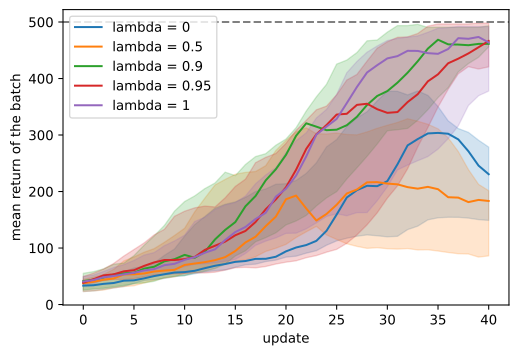
for lam, r in sweep.items():
    best = np.array([np.convolve(c, np.ones(20) / 20, 'valid').max()
                     for c in r])
    print(f'lambda = {lam:4}: best 20-update window, '
          f'median {np.median(best):5.1f}, seeds {np.round(np.sort(best))}')
d2l.plot_curves({f'lambda = {lam:g}': r for lam, r in sweep.items()},
                xlabel='update', ylabel='mean return of the batch',
                smooth=10, reference=500)
lambda = 0.0: best 20-update window, median 161.9, seeds [144. 145. 162. 302. 474.]
lambda = 0.5: best 20-update window, median 201.3, seeds [174. 183. 201. 312. 371.]
lambda = 0.9: best 20-update window, median 322.5, seeds [274. 319. 322. 488. 492.]
lambda = 0.95: best 20-update window, median 460.6, seeds [348. 372. 461. 486. 497.]
lambda = 1.0: best 20-update window, median 466.2, seeds [415. 456. 466. 469. 497.]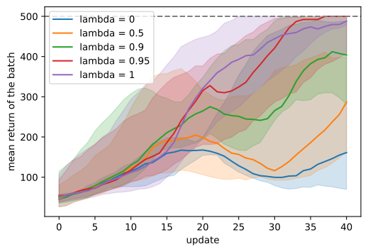
The \(\lambda=0\) and \(\lambda=0.5\) runs remain far below the maximum return when the 50-update budget ends, whereas the seed ranges for \(\lambda\geq0.9\) overlap. Early in training, the critic is inaccurate, so estimators that depend less on it improve faster. The longer comparison above showed the complementary result: after the critic improves, the \(\lambda=0\) runs have the longest consecutive intervals at the maximum return.
Training curves combine estimator quality with optimization and changing data. To examine the estimator directly, we freeze a partially trained agent and draw many batches at fixed parameters. For each \(\lambda\), we compare the resulting policy-gradient estimates with a reference.
The reference is the mean of the \(\lambda=1\) estimator over all draws. It approximates the unbiased Monte Carlo gradient without requiring a solvable model, although it remains subject to finite-sample error.
rng, env = np.random.default_rng(1), gym.make('CartPole-v1')
frozen = cartpole_agent(1)
env.reset(seed=1)
for _ in range(40):   # a mid-training freeze: the critic is still wrong
    b = d2l.rollout(env, frozen.act, batch_episodes, rng)
    for _ in range(critic_steps):
        fit_value(frozen, b.obs, b.td_target(frozen.value_np, gamma))
    policy_step_clip(frozen, b, d2l.normalize(
        b.td_target(frozen.value_np, gamma) - frozen.value_np(b.obs)))
rng, env = np.random.default_rng(1), gym.make('CartPole-v1')
frozen = cartpole_agent(1)
env.reset(seed=1)
for _ in range(40): # a mid-training freeze: the critic is still wrong
b = d2l.rollout(env, frozen.act, batch_episodes, rng)
for _ in range(critic_steps):
fit_value(frozen, b.obs, b.td_target(frozen.value_np, gamma))
policy_step_clip(frozen, b, d2l.normalize(
b.td_target(frozen.value_np, gamma) - frozen.value_np(b.obs)))if tab.selected('pytorch'):
def grad_vec(ac, b, w):
loss = -(torch.as_tensor(w) * ac.log_prob(
torch.as_tensor(b.obs), torch.as_tensor(b.act))).mean()
g = torch.autograd.grad(loss, list(ac.policy.parameters()))
return np.concatenate([x.numpy().ravel() for x in g])
if tab.selected('jax'):
@nnx.jit
def _grad_tree(policy, obs, act, adv, n_real):
return nnx.grad(lambda p: -(adv * jax.nn.log_softmax(p(obs), -1)[
jnp.arange(obs.shape[0]), act]).sum() / n_real)(policy)
def grad_vec(ac, b, w): # padded + jitted: 1000 calls below
size = 1 << max(6, (len(w) - 1).bit_length())
g = _grad_tree(ac.policy, _pad(b.obs, size), _pad(b.act, size),
_pad(w, size), jnp.float32(len(w)))
return np.concatenate([np.asarray(x).ravel()
for x in jax.tree.leaves(g)])
draws = {lam: [] for lam in lams}
for _ in range(200):
b = d2l.rollout(env, frozen.act, 4, rng)
for lam in lams:
draws[lam].append(grad_vec(frozen, b,
b.gae(frozen.value_np, gamma, lam)))
u_ref = np.stack(draws[1.0]).mean(axis=0) # the many-rollout reference
for lam in lams:
u = np.stack(draws[lam])
bias = np.linalg.norm(u.mean(0) - u_ref) / np.linalg.norm(u_ref)
var = ((u - u.mean(0)) ** 2).sum(1).mean() / (u_ref ** 2).sum()
print(f'lambda = {lam:4}: relative bias {bias:4.2f}, relative '
f'variance {var:6.1f}, one-draw error {bias ** 2 + var:6.1f}')lambda = 0.0: relative bias 1.05, relative variance 0.1, one-draw error 1.2
lambda = 0.5: relative bias 1.06, relative variance 0.1, one-draw error 1.2
lambda = 0.9: relative bias 0.95, relative variance 0.2, one-draw error 1.1
lambda = 0.95: relative bias 0.83, relative variance 0.3, one-draw error 0.9
lambda = 1.0: relative bias 0.00, relative variance 1.6, one-draw error 1.6if tab.selected('pytorch'):
def grad_vec(ac, b, w):
loss = -(torch.as_tensor(w) * ac.log_prob(
torch.as_tensor(b.obs), torch.as_tensor(b.act))).mean()
g = torch.autograd.grad(loss, list(ac.policy.parameters()))
return np.concatenate([x.numpy().ravel() for x in g])
if tab.selected('jax'):
@nnx.jit
def _grad_tree(policy, obs, act, adv, n_real):
return nnx.grad(lambda p: -(adv * jax.nn.log_softmax(p(obs), -1)[
jnp.arange(obs.shape[0]), act]).sum() / n_real)(policy)
def grad_vec(ac, b, w): # padded + jitted: 1000 calls below
size = 1 << max(6, (len(w) - 1).bit_length())
g = _grad_tree(ac.policy, _pad(b.obs, size), _pad(b.act, size),
_pad(w, size), jnp.float32(len(w)))
return np.concatenate([np.asarray(x).ravel()
for x in jax.tree.leaves(g)])
draws = {lam: [] for lam in lams}
for _ in range(200):
b = d2l.rollout(env, frozen.act, 4, rng)
for lam in lams:
draws[lam].append(grad_vec(frozen, b,
b.gae(frozen.value_np, gamma, lam)))
u_ref = np.stack(draws[1.0]).mean(axis=0) # the many-rollout reference
for lam in lams:
u = np.stack(draws[lam])
bias = np.linalg.norm(u.mean(0) - u_ref) / np.linalg.norm(u_ref)
var = ((u - u.mean(0)) ** 2).sum(1).mean() / (u_ref ** 2).sum()
print(f'lambda = {lam:4}: relative bias {bias:4.2f}, relative '
f'variance {var:6.1f}, one-draw error {bias ** 2 + var:6.1f}')lambda = 0.0: relative bias 1.34, relative variance 0.3, one-draw error 2.1
lambda = 0.5: relative bias 1.22, relative variance 0.4, one-draw error 1.9
lambda = 0.9: relative bias 0.57, relative variance 1.4, one-draw error 1.7
lambda = 0.95: relative bias 0.26, relative variance 2.4, one-draw error 2.5
lambda = 1.0: relative bias 0.00, relative variance 5.9, one-draw error 5.9Moving from \(\lambda=1\) toward smaller values first reduces variance rapidly; most of the reduction has occurred by \(\lambda=0.9\). Bias increases more gradually toward \(\lambda=0\). The estimated one-draw error, bias squared plus variance, is therefore large at both endpoints and smallest between \(\lambda=0.9\) and \(0.95\) in these experiments. Common PPO implementations use values in this range (Section 15.2).
The location is not universal. It depends on the accuracy of the frozen critic and on the task. Moreover, the \(\lambda=1\) row has zero estimated bias by construction because its sample mean defines the reference.
The reference itself is estimated from 200 draws of the highest-variance estimator. The bias column is therefore reliable only for differences large relative to this finite-sample error; the reported large-\(\lambda\) differences satisfy that condition.
Finally, we evaluate the trained policies from seed 0 greedily, removing action-sampling variability from the comparison.
env = gym.make('CartPole-v1')
for name in runs:
    env.reset(seed=2)
    score = d2l.evaluate(env, agents[name][0].act_greedy, num_episodes=100)
    print(f'{name:>20}: greedy mean return over 100 episodes: {score:.0f}')
REINFORCE + baseline: greedy mean return over 100 episodes: 500
actor-critic: greedy mean return over 100 episodes: 500env = gym.make('CartPole-v1')
for name in runs:
env.reset(seed=2)
score = d2l.evaluate(env, agents[name][0].act_greedy, num_episodes=100)
print(f'{name:>20}: greedy mean return over 100 episodes: {score:.0f}')REINFORCE + baseline: greedy mean return over 100 episodes: 499
actor-critic: greedy mean return over 100 episodes: 500Both agents finish at 499 or 500, so this experiment does not rank their final policies. It instead compares estimator variance, gradient norms, and the persistence of ceiling-level batches during training.
15.1.5 Summary
Actor–critic methods use a learned value function to construct bootstrapped policy-gradient weights. With an exact critic, the expected temporal-difference error equals the advantage; an approximate critic introduces bias while usually reducing variance. The critic update is a semi-gradient policy-evaluation step, and the actor and critic form an approximate generalized policy-iteration scheme. Multi-step returns interpolate between one-step bootstrapping and Monte Carlo returns. The \(\lambda\)-return mixes these targets geometrically, and GAE computes the equivalent discounted sum of temporal-difference errors with a backward scan.
Experimental scope. The training comparisons use three seeds per framework, the \(\lambda\) sweep uses five seeds, and the frozen-policy estimator study uses 200 batches. Both one-step and Monte Carlo methods solve CartPole in these runs. Intermediate high values of \(\lambda\) give the smallest estimator error on the frozen-policy probe, but the precise optimum varies by framework and policy. The experiments support the bias–variance interpretation rather than a universal choice of \(\lambda\).
15.1.6 Exercises
- [conceptual] Why the baseline argument does not extend. The identity of Section 14.6 allowed any \(b(s_t)\) to be subtracted from the weight without bias. Explain why it does not cover the bootstrapped weight \(\delta_t\) of Equation 15.1.2, by pointing at exactly which quantity in the argument stops being independent of the action \(a_t\). Under what condition on \(\hat{V}\) does the bias vanish?
- [short-code] Where the U comes from. Take the estimator table’s relative bias and variance per \(\lambda\) and combine them into a predicted single-draw error, then predict which \(\lambda\) the training sweep should favor before looking at its returns. Where prediction and sweep disagree, what does the disagreement say about what a training run adds that a frozen-policy estimate cannot see? (The critic improves during training, the policy moves, and the weight scale interacts with the step size.)
- [short-code] The two timescales. Sweep
critic_stepsover \(\{1, 5, 20\}\), two seeds each; about twenty minutes on a laptop CPU. Where does the algorithm fail, and does it fail by learning nothing or by learning something wrong? Connect the failure to the sentence in the two-timescale paragraph about the critic chasing a moving target twice over. - [short-code] The clip, removed. Log the norm of the policy gradient in both methods, before the clip is applied. Although both normalize their weights to unit variance, the actor-critic norms come out roughly an order of magnitude larger. Explain the gap with the baseline argument of Section 14.6, then predict, and check, which of the two runs changes at all when
grad_clipis removed. - [extended] Fully online. Equation 15.1.3 can be applied at every single transition, with no batch at all. Implement this variant on CartPole and compare it with the batched version at a matched number of environment steps. What goes wrong, and which ingredient of Section 15.4’s recipe addresses it?
- [conceptual] Where the actor-critic sits. Place REINFORCE, REINFORCE with a learned baseline, actor-critic, and Q-learning on two axes: how much bias the update carries, and how long the algorithm must wait before it can learn from a transition. Which corner is empty, and why?