%matplotlib inline
from d2l import torch as d2l
import torch2.4 Linear Regression Implementation from Scratch
This section implements linear regression using only tensors and automatic differentiation. The implementation has four components: the linear model, the squared loss, minibatch stochastic gradient descent, and the training loop. We apply them to the synthetic dataset from Section 2.3, where the known parameters allow us to check the result directly.
Writing these components explicitly makes their interfaces and interactions visible. The next section expresses the same computation using the reusable layers, losses, optimizers, and data loaders supplied by each framework.
%matplotlib inline
from d2l import tensorflow as d2l
import tensorflow as tf%matplotlib inline
from d2l import jax as d2l
from flax import nnx
import jax
from jax import numpy as jnp
import optax%matplotlib inline
from d2l import mxnet as d2l
from mxnet import autograd, np, npx
npx.set_np()2.4.1 Defining the Model
Before we can begin optimizing our model’s parameters by minibatch SGD, we need to have some parameters in the first place. In the following we initialize weights by drawing random numbers from a normal distribution with mean 0 and a standard deviation of 0.01. For this convex linear model, a small nonzero scale such as 0.01 is sufficient to start optimization and is not a general initialization prescription. The argument sigma exposes the choice; variance-preserving schemes for deep networks are developed in Section 4.4. Moreover we set the bias to 0. Note that for object-oriented design we add the code to the __init__ method of a subclass of d2l.Module (introduced in Section 2.2.2).
class LinearRegressionScratch(d2l.Module):
    """The linear regression model implemented from scratch."""
    def __init__(self, num_inputs, lr, sigma=0.01):
        super().__init__()
        self.save_hyperparameters()
        self.w = d2l.normal(0, sigma, (num_inputs, 1), requires_grad=True)
        self.b = d2l.zeros(1, requires_grad=True)
class LinearRegressionScratch(d2l.Module):
"""The linear regression model implemented from scratch."""
def __init__(self, num_inputs, lr, sigma=0.01):
super().__init__()
self.save_hyperparameters()
w = tf.random.normal((num_inputs, 1), mean=0, stddev=0.01)
b = tf.zeros(1)
self.w = tf.Variable(w, trainable=True)
self.b = tf.Variable(b, trainable=True)class LinearRegressionScratch(d2l.Module):
"""The linear regression model implemented from scratch."""
def __init__(self, num_inputs, lr, sigma=0.01, rngs=None):
super().__init__()
self.save_hyperparameters(ignore=['rngs'])
rngs = nnx.Rngs(d2l.get_key()) if rngs is None else rngs
self.w = nnx.Param(
rngs.params.normal((num_inputs, 1)) * sigma)
self.b = nnx.Param(jnp.zeros(1))class LinearRegressionScratch(d2l.Module):
"""The linear regression model implemented from scratch."""
def __init__(self, num_inputs, lr, sigma=0.01):
super().__init__()
self.save_hyperparameters()
self.w = d2l.normal(0, sigma, (num_inputs, 1))
self.b = d2l.zeros(1)
self.w.attach_grad()
self.b.attach_grad()We next define how the model maps its inputs and parameters to its output. Using the notation of Equation 2.1.3, the linear model takes the matrix–vector product of the input features \(\mathbf{X}\) and the model weights \(\mathbf{w}\), and add the offset \(b\) to each example. The product \(\mathbf{Xw}\) is a vector and \(b\) is a scalar. Because of the broadcasting mechanism (see Section 1.1.4), when we add a vector and a scalar, the scalar is added to each component of the vector. The resulting forward method is registered in the LinearRegressionScratch class via add_to_class (introduced in Section 2.2.1).
@d2l.add_to_class(LinearRegressionScratch)
def forward(self, X):
    return d2l.matmul(X, self.w) + self.b
2.4.2 Defining the Loss Function
Since updating our model requires taking the gradient of our loss function, we ought to define the loss function first. Here we use the squared loss function in Equation 2.1.4. Our synthetic data loader already yields labels y with the same shape as the predictions y_hat (both are \((B, 1)\) column vectors for a batch of size \(B\)), so we can subtract them elementwise directly; exercise 5 asks what would go wrong if the two shapes did not match. We return the averaged loss value among all examples in the minibatch.
@d2l.add_to_class(LinearRegressionScratch)
def loss(self, y_hat, y):
    l = (y_hat - y) ** 2 / 2
return d2l.reduce_mean(l)@d2l.add_to_class(LinearRegressionScratch)
def loss(self, y_hat, y):
l = (y_hat - y) ** 2 / 2
return d2l.reduce_mean(l)@d2l.add_to_class(LinearRegressionScratch)
def loss(self, y_hat, y):
l = (y_hat - d2l.reshape(y, y_hat.shape)) ** 2 / 2
return d2l.reduce_mean(l)@d2l.add_to_class(LinearRegressionScratch)
def loss(self, y_hat, y):
l = (y_hat - y) ** 2 / 2
return d2l.reduce_mean(l)Before handing this loss to an optimizer, compute by hand the gradient that the optimizer will consume. For a single example, the loss is \(\ell = \frac{1}{2}(\hat{y} - y)^2\) with \(\hat{y} = \mathbf{w}^\top \mathbf{x} + b\), and the chain rule gives
\[\frac{\partial \ell}{\partial \mathbf{w}} = (\hat{y} - y)\, \mathbf{x} \qquad \textrm{and} \qquad \frac{\partial \ell}{\partial b} = \hat{y} - y. \tag{2.4.1}\]
Differentiating the square produces the error \(\hat{y} - y\), which is then multiplied by the derivative of \(\hat{y}\) with respect to each parameter: \(\mathbf{x}\) for the weights and \(1\) for the bias. In words, the gradient is the error-weighted input: each weight \(w_j\) receives a gradient proportional to the residual and to \(x_j\), while the bias gradient equals the residual. Averaging these per-example gradients over a minibatch recovers exactly the closed-form update we wrote down in Equation 2.1.9. The backward pass stores this averaged gradient in each parameter’s gradient field, which the SGD class below reads through param.grad.
2.4.3 Defining the Optimization Algorithm
As discussed in Section 2.1, linear regression has a closed-form solution. Our purpose here is to establish the minibatch SGD procedure used to train models that lack a closed-form solution. At each step, using a minibatch randomly drawn from our dataset, we estimate the gradient of the loss with respect to the parameters. Next, we subtract a scaled gradient; for a suitable learning rate, this direction locally reduces the loss.
The following code applies the update, given a set of parameters, and a learning rate lr. Since our loss is computed as an average over the minibatch, we do not need to adjust the learning rate against the batch size. In later chapters we will investigate how learning rates should be adjusted for very large minibatches as they arise in distributed large-scale learning. For now, we can ignore this dependency.
We define our SGD class, a subclass of d2l.HyperParameters (introduced in Section 2.2.1), to have a similar API as the built-in SGD optimizer. We update the parameters in the step method. The zero_grad method sets all gradients to 0, which must be run before a backpropagation step.
We define our SGD class, a subclass of d2l.HyperParameters (introduced in Section 2.2.1), to have a similar API as the built-in SGD optimizer. We update the parameters in the apply_gradients method. It accepts a list of parameter and gradient pairs.
We define our SGD class, a subclass of d2l.HyperParameters (introduced in Section 2.2.1), to have a similar API as the built-in SGD optimizer. We update the parameters in the step method. It accepts a batch_size argument that can be ignored.
class SGD(d2l.HyperParameters):
    """Minibatch stochastic gradient descent."""
    def __init__(self, params, lr):
        self.save_hyperparameters()

    def step(self):
        for param in self.params:
            param -= self.lr * param.grad

    def zero_grad(self):
        for param in self.params:
            if param.grad is not None:
                param.grad.zero_()
class SGD(d2l.HyperParameters):
"""Minibatch stochastic gradient descent."""
def __init__(self, lr):
self.save_hyperparameters()
def apply_gradients(self, grads_and_vars):
for grad, param in grads_and_vars:
param.assign_sub(self.lr * grad)class SGD(d2l.HyperParameters):
"""Minibatch stochastic gradient descent."""
# The key transformation of Optax is the GradientTransformation
# defined by two methods, the init and the update.
# The init initializes the state and the update transforms the gradients.
# https://github.com/deepmind/optax/blob/master/optax/_src/transform.py
def __init__(self, lr):
self.save_hyperparameters()
def init(self, params):
# Delete unused params
del params
# Return an EmptyState *instance* (an empty NamedTuple, hence a valid
# pytree) -- not the class -- so this hand-rolled optimizer is
# JIT-traceable just like any optax GradientTransformation.
return optax.EmptyState()
def update(self, updates, state, params=None):
del params
# NNX's Optimizer applies these updates to its model's parameters.
updates = jax.tree_util.tree_map(lambda g: -self.lr * g, updates)
return updates, state
def __call__(self):
return optax.GradientTransformation(self.init, self.update)class SGD(d2l.HyperParameters):
"""Minibatch stochastic gradient descent."""
def __init__(self, params, lr):
self.save_hyperparameters()
def step(self, _):
for param in self.params:
param -= self.lr * param.gradEvery optimization step has a forward pass and loss, a backward pass that stores each parameter’s minibatch-average gradient \(\partial L/\partial
\theta\), and an in-place update that subtracts \(\eta\) times that gradient. Two ordering constraints matter. First, if the backward pass accumulates into whatever gradient is already stored (Section 1.5), those buffers must be cleared before it runs, or a leftover gradient from the previous minibatch contaminates this one. Second, the update must run last and outside the gradient graph, so that the subtraction is not itself differentiated and does not extend the graph; this is why it sits under a no-tracking guard. Without clearing, the next backward pass includes gradients from earlier minibatches. Without the guard, the update may raise an error or extend the computation graph. The fit_epoch method applies this sequence to each minibatch.
We next define the configure_optimizers method, which returns an instance of the SGD class.
@d2l.add_to_class(LinearRegressionScratch)
def configure_optimizers(self):
return SGD([self.w, self.b], self.lr)@d2l.add_to_class(LinearRegressionScratch)
def configure_optimizers(self):
return SGD(self.lr)@d2l.add_to_class(LinearRegressionScratch)
def configure_optimizers(self):
return SGD(self.lr)@d2l.add_to_class(LinearRegressionScratch)
def configure_optimizers(self):
return SGD([self.w, self.b], self.lr)2.4.4 Training
The parameters, loss, model, and optimizer now define one minibatch update. The training loop repeats that update over every batch and records its progress; the same ordering constraints recur in later models. In each epoch, we iterate through the entire training dataset, passing once through every example (up to a final partial batch when the number of examples is not divisible by the batch size). In each iteration, we grab a minibatch of training examples, and compute its loss through the model’s training_step method. Then we compute the gradients with respect to each parameter. Finally, we will call the optimization algorithm to update the model parameters. In summary, we will execute the following loop:
- Initialize parameters \((\mathbf{w}, b)\)
- Repeat until done
- Compute gradient \(\mathbf{g} \leftarrow \partial_{(\mathbf{w},b)} \frac{1}{|\mathcal{B}|} \sum_{i \in \mathcal{B}} l(\mathbf{x}^{(i)}, y^{(i)}, \mathbf{w}, b)\)
- Update parameters \((\mathbf{w}, b) \leftarrow (\mathbf{w}, b) - \eta \mathbf{g}\)
Recall that the synthetic regression data module that we generated in Section 2.3 holds out 1000 validation examples alongside the training data. We will almost always want such a validation dataset to measure our model quality. Here we pass the validation dataloader once in each epoch to measure the model performance. Following our object-oriented design, the prepare_batch and fit_epoch methods are registered in the d2l.Trainer class (introduced in Section 2.2.4).
In TensorFlow, executing each operation one at a time from Python is much slower than having the framework run an entire sequence of operations as one compiled graph. We therefore use tf.function to compile the forward pass, loss computation, gradient calculation, and parameter update into a single fused step. This happens in _compile_steps, which is called once at the beginning of training. Since tf.function traces through Python code to build a static graph, side effects like plotting cannot live inside it. We thus split each step into a compiled part (_train_step, _val_step) that does the heavy computation, and a reporting part (_report_train, _report_val) that records metrics in Python. Before tracing, we run one forward pass to let Keras create the layer weights, since tf.function needs all variables to exist at trace time. The graph-compilation cost is paid once per trace; its benefit over running the same operations one at a time from Python grows with model and batch size.
JAX traces pure functions, while NNX manages the associated object state: the module owns its parameters, and nnx.value_and_grad differentiates the loss with respect to the module itself. Running each operation one at a time from Python would pay a dispatch cost on every call; compiling the whole step removes it. We therefore wrap one training step — forward, loss, gradients, and the in-place optimizer.update(model, grads) — in a single @nnx.jit function, _trainer_train_step, with a companion _trainer_validation_step for evaluation. nnx.jit splits the module into static structure and mutable state at the compilation boundary and stitches the updated state back afterwards, so the entire per-batch work is one compiled call, and the mutation you see in the Python code is exactly what happens.
@d2l.add_to_class(d2l.Trainer)
def prepare_batch(self, batch):
return batch@d2l.add_to_class(d2l.Trainer)
def fit_epoch(self):
self.model.train()
for batch in self.train_dataloader:
loss = self.model.training_step(self.prepare_batch(batch))
self.optim.zero_grad()
loss.backward()
if self.gradient_clip_val > 0: # To be discussed later
self.clip_gradients(self.gradient_clip_val, self.model)
# The `no_grad` only needs to wrap the parameter update; the
# scratch `SGD.step` does an in-place `param -= lr * grad`,
# which would otherwise be flagged as a leaf-tensor mutation.
with torch.no_grad():
self.optim.step()
self.train_batch_idx += 1
if self.val_dataloader is None:
return
self.model.eval()
for batch in self.val_dataloader:
with torch.no_grad():
self.model.validation_step(self.prepare_batch(batch))
self.val_batch_idx += 1@d2l.add_to_class(d2l.Trainer)
def _compile_steps(self):
model, optim = self.model, self.optim
grad_clip = self.gradient_clip_val
for batch in self.train_dataloader:
model(*self.prepare_batch(batch)[:-1], training=True)
break
def train_step(batch):
with tf.GradientTape() as tape:
loss = model.loss(model(*batch[:-1], training=True),
batch[-1])
params = model.trainable_variables
if not params:
params = list(tape.watched_variables())
grads = tape.gradient(loss, params)
if grad_clip > 0:
grads = self.clip_gradients(grad_clip, grads)
optim.apply_gradients(zip(grads, params))
return loss
def val_step(batch):
return model(*batch[:-1], training=False)
train_step = tf.function(train_step, reduce_retracing=True)
val_step = tf.function(val_step, reduce_retracing=True)
self._train_step = train_step
self._val_step = val_step
@d2l.add_to_class(d2l.Trainer)
def fit_epoch(self):
self.model.training = True
for batch in self.train_dataloader:
loss = self._train_step(self.prepare_batch(batch))
self.model._report_train(loss)
self.train_batch_idx += 1
if self.val_dataloader is None:
return
self.model.training = False
for batch in self.val_dataloader:
b = self.prepare_batch(batch)
y_hat = self._val_step(b)
self.model._report_val(y_hat, b)
self.val_batch_idx += 1@nnx.jit
def _trainer_train_step(model, optimizer, batch):
loss, grads = nnx.value_and_grad(
lambda m: m.training_step(batch))(model)
optimizer.update(model, grads)
return loss
@nnx.jit
def _trainer_validation_step(model, batch):
return model.validation_step(batch)
@d2l.add_to_class(d2l.Trainer)
def fit_epoch(self):
for batch in self.train_dataloader:
loss = _trainer_train_step(
self.train_model, self.optim, self.prepare_batch(batch))
self.model.plot('loss', loss, train=True)
self.train_batch_idx += 1
if self.val_dataloader is None:
return
for batch in self.val_dataloader:
metrics = _trainer_validation_step(
self.val_model, self.prepare_batch(batch))
if isinstance(metrics, tuple):
loss, accuracy = metrics
self.model.plot('acc', accuracy, train=False)
else:
loss = metrics
self.model.plot('loss', loss, train=False)
self.val_batch_idx += 1@d2l.add_to_class(d2l.Trainer)
def fit_epoch(self):
for batch in self.train_dataloader:
with autograd.record():
loss = self.model.training_step(self.prepare_batch(batch))
loss.backward()
if self.gradient_clip_val > 0:
self.clip_gradients(self.gradient_clip_val, self.model)
self.optim.step(1)
self.train_batch_idx += 1
if self.val_dataloader is None:
return
for batch in self.val_dataloader:
self.model.validation_step(self.prepare_batch(batch))
self.val_batch_idx += 1We are almost ready to train the model, but first we need some training data. Here we use the SyntheticRegressionData class and pass in some ground truth parameters. Then we train our model with the learning rate lr=0.03 and set max_epochs=10. Note that in general, both the number of epochs and the learning rate are hyperparameters. Setting hyperparameters is tricky and we will usually want to use a three-way split, one set for training, a second for hyperparameter selection, and the third reserved for the final evaluation. We elide these details for now and develop model selection, validation, and the train/validation/test split in Section 2.6.
So that repeated runs of this notebook produce identical numbers, we first fix the seed of the framework’s random number generator, which governs both the parameter initialization and the shuffling of minibatches.
JAX needs no such call: its PRNG is functional, with no implicit global state. The model and dataset receive explicit typed keys; the synthetic dataset defaults to key=jax.random.key(0). Reusing a key repeats the same random draw, so stochastic programs should split and thread keys explicitly; see exercise 4 of Section 2.3.
torch.manual_seed(1)<torch._C.Generator at 0x78330bbd6530>tf.random.set_seed(1)npx.random.seed(1)model = LinearRegressionScratch(2, lr=0.03)
data = d2l.SyntheticRegressionData(w=d2l.tensor([2, -3.4]), b=4.2)
trainer = d2l.Trainer(max_epochs=10)
trainer.fit(model, data)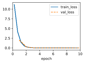
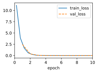
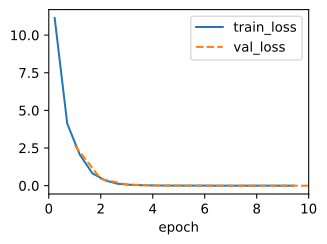
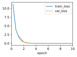
The fit call above produces a live plot of the training and validation loss against the epoch. Both curves fall together and flatten near the irreducible noise floor (with \(\sigma = 0.01\) the per-example squared loss bottoms out around \(\sigma^2/2 \approx 5\times 10^{-5}\)). In this run, the validation curve closely tracks the training curve. That small gap is consistent with fitting a low-capacity model to 1000 examples. We return to the train/validation gap, and what to do when it opens, in Section 2.6.
Because we synthesized the dataset ourselves, we know precisely what the true parameters are. Thus, we can evaluate our success in training by comparing the true parameters with those that we learned through our training loop. Indeed they turn out to be very close to each other.
with torch.no_grad():
    print(f'error in estimating w: {data.w - d2l.reshape(model.w, data.w.shape)}')
    print(f'error in estimating b: {data.b - model.b}')
error in estimating w: tensor([ 3.5524e-05, -3.0398e-04])
error in estimating b: tensor([0.0003])print(f'error in estimating w: {data.w - d2l.reshape(model.w, data.w.shape)}')
print(f'error in estimating b: {data.b - model.b}')error in estimating w: [ 2.6345253e-05 -4.0531158e-06]
error in estimating b: [-0.00025082]print(f"error in estimating w: "
f"{data.w - d2l.reshape(model.w[...], data.w.shape)}")
print(f"error in estimating b: {data.b - model.b[...]}")error in estimating w: [ 0.00044107 -0.00051808]
error in estimating b: [0.00095987]print(f'error in estimating w: {data.w - d2l.reshape(model.w, data.w.shape)}')
print(f'error in estimating b: {data.b - model.b}')error in estimating w: [ 2.8300285e-04 -7.5340271e-05]
error in estimating b: [0.0002408]We should not take the ability to exactly recover the ground truth parameters for granted. In general, for deep models unique solutions for the parameters do not exist, and even for linear models, exactly recovering the parameters is only possible when no feature is linearly dependent on the others. However, in machine learning, we are often less concerned with recovering true underlying parameters than with finding parameters that lead to highly accurate prediction (Vapnik 1992). Even on difficult optimization problems, stochastic gradient descent can often find parameters with low training loss, owing partly to the fact that, for deep networks, there exist many configurations of the parameters that lead to highly accurate prediction. Explaining why some solutions found by SGD also generalize well remains an active research problem, taken up in Section 4.5.
2.4.5 Summary
We implemented the data loader, linear model, squared loss, stochastic gradient update, and training loop explicitly. Their separation makes the training procedure easy to inspect and modify. Framework implementations can replace these components with optimized abstractions while retaining the same computational structure.
The hand-rolled SGD above is the simplest member of a large family: momentum, AdaGrad, RMSProp, and Adam all replace that single update line, and learning-rate schedules anneal \(\eta\) over the course of training; these are developed in Chapter 9. The squared loss, likewise, is a modelling choice; in Section 2.7 we add a penalty on \(\|\mathbf{w}\|\) to curb overfitting, the first of many regularizers we will meet.
2.4.6 Exercises
Initialization at the extremes. Predict whether training still succeeds if the weights are initialized to exactly zero, and separately if they are initialized with variance \(1000\) rather than \(0.01\). Explain both answers, noting that this model is a single linear layer rather than a deep network.
[code] Ohm’s law. Assume that you are Georg Simon Ohm trying to come up with a model for resistance that relates voltage and current. Treat the resistance as a learnable parameter and fit it to voltage–current pairs using this section’s autograd-based training loop.
[code] Planck’s law. ● Use Planck’s Law to determine the temperature of an object from its spectral energy density. For reference, the spectral density \(B\) of radiation emanating from a black body is
\[B(\lambda, T) = \frac{2 hc^2}{\lambda^5} \cdot \left(\exp \frac{h c}{\lambda k T} - 1\right)^{-1}, \tag{2.4.2}\]
where \(\lambda\) is the wavelength, \(T\) is the temperature, \(c\) is the speed of light, \(h\) is Planck’s constant, and \(k\) is the Boltzmann constant. Given measured energies at several wavelengths, fit the temperature \(T\) as a learnable parameter under this section’s training loop.
Second derivatives. Identify the problems you would encounter if you wanted to compute the second derivatives of the loss with the tools introduced so far, and propose how to fix them.
Reshape in the loss. Explain what silently goes wrong in the loss computation if
y_hatandyhave mismatched shapes: the failure comes from broadcasting, not from an error message.[code] Learning-rate sweep. Train the from-scratch model at each learning rate in \(\{0.001, 0.01, 0.03, 0.1, 0.3, 1.0\}\) for a fixed 30 epochs and plot the training-loss curves. For each rate, report the smallest number of epochs needed to come within 10% of the noise floor \(\sigma^2/2\), marking rates that diverge or never reach that band.
Adapted from Andrew Ng’s Coursera Machine Learning, exercise 1.
[code] Robust losses. Implement the absolute value loss
(y_hat - d2l.reshape(y, y_hat.shape)).abs().mean(). If you sum rather than average, the gradient scales with the batch size, so you must lower the learning rate to compensate.- Check what happens for regular data.
- Check whether there is a difference in behavior if you actively perturb some entries of \(\mathbf{y}\), such as \(y_5 = 10000\).
- Design a cheap loss that combines the best aspects of squared loss and absolute value loss, quadratic near zero and linear in the tails. Confirm that it recovers a fit close to the uncorrupted case even after the perturbation.
Why reshuffle. Explain why each epoch reshuffles the dataset. Then construct a small dataset ordering, for example sorted by label, that would break minibatch SGD if reshuffling were disabled, and state specifically how it breaks.