%matplotlib inline
from d2l import torch as d2l
import gymnasium as gym
import numpy as np15.6 On-Policy, Off-Policy, and Offline Learning
On-policy estimators require data from the current policy, whereas off-policy value methods can use transitions collected by other policies. This distinction determines whether a batch may be reused and whether learning from a fixed dataset is possible. We first compare the Q-learning and SARSA targets to make the distinction explicit.
In offline reinforcement learning, the agent receives a fixed dataset and cannot collect additional transitions. Errors on poorly covered actions are therefore not corrected by subsequent interaction. Using tabular FrozenLake, where the optimal value is known, we measure this extrapolation error and examine a count-based pessimistic penalty. The example also clarifies the difference between improving predicted value and improving the policy’s delivered return.
%matplotlib inline
from d2l import jax as d2l
import gymnasium as gym
import numpy as np
15.6.1 On-Policy and Off-Policy Updates
15.6.1.1 The Two Families of Update Rules
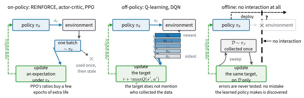
The update rules of the last two chapters fall into two families. A policy gradient is an expectation under the current policy’s trajectory distribution, so samples from another policy generally estimate a different quantity. REINFORCE and actor-critic are therefore on-policy; PPO permits limited reuse by correcting action probabilities. By contrast, the Q-learning target \(r + \gamma \max_{a'} \hat{Q}(s', a')\) depends on the environment transition but not on the policy that selected \(a\). A transition collected by an earlier policy, another agent, or a fixed log is therefore a valid sample of the same Bellman backup. This is off-policy learning. Figure 15.6.1 compares these cases with the offline setting introduced below.
15.6.1.2 SARSA: Bootstrapping on the Action Taken
SARSA differs from Q-learning in the action used for bootstrapping. In the update from Equation 14.4.4, replace the best action at \(s'\) by the action \(a'\) actually selected by the behavior policy:
\[\delta_{\textrm{SARSA}} = r + \gamma\, Q(s', a') - Q(s, a), \tag{15.6.1}\]
The quintuple \((s,a,r,s',a')\) gives SARSA its name (Rummery and Niranjan 1994). In Figure 14.2.1, its update is panel (d) without the arc denoting maximization: the target follows the sampled action \(a'\).
Averaging this target over \(a'\sim\pi_e(\cdot\mid s')\) yields the Bellman expectation backup for the behavior policy \(\pi_e\). For a stationary behavior policy, SARSA therefore converges to \(Q^{\pi_e}\), whereas Q-learning targets \(Q^*\) independently of the behavior policy. During learning, our \(\epsilon\)-greedy behavior changes with the table, so we compare the final table with the value of the final frozen policy. The following implementation runs both algorithms on the slippery lake with \(\epsilon=0.3\); only the bootstrap action differs:
gamma, epsilon = 0.95, 0.3            # discount; the fixed exploration rate
num_episodes, num_datasets = 500, 15  # episodes per dataset; dataset draws
num_sweeps, alpha, kappa = 200, 0.2, 0.1  # offline sweeps; step; pessimism
env = gym.make('FrozenLake-v1', is_slippery=True)
mdp = d2l.TabularMDP.from_gym(env, gamma)
gamma, epsilon = 0.95, 0.3 # discount; the fixed exploration rate
num_episodes, num_datasets = 500, 15 # episodes per dataset; dataset draws
num_sweeps, alpha, kappa = 200, 0.2, 0.1 # offline sweeps; step; pessimism
env = gym.make('FrozenLake-v1', is_slippery=True)
mdp = d2l.TabularMDP.from_gym(env, gamma)def td_control(seed, env, num_episodes, epsilon, on_policy):
"""Q-learning and SARSA in one loop: they differ in a single symbol."""
rng = np.random.default_rng(seed)
Q, visits = np.zeros((16, 4)), np.zeros((16, 4))
env.reset(seed=seed)
for _ in range(num_episodes):
s, done = env.reset()[0], False
a = d2l.epsilon_greedy(Q[s], epsilon, rng)
while not done:
s2, r, terminated, truncated, _ = env.step(a)
a2 = d2l.epsilon_greedy(Q[s2], epsilon, rng)
target = Q[s2, a2] if on_policy else Q[s2].max() # the symbol
visits[s, a] += 1
Q[s, a] += (r + gamma * (1 - terminated) * target
- Q[s, a]) / (1 + 0.1 * visits[s, a])
s, a, done = s2, a2, terminated or truncated
return Q
Q_q = td_control(0, env, 8000, epsilon, on_policy=False)
Q_sarsa = td_control(0, env, 8000, epsilon, on_policy=True)
d2l.show_grid(env.unwrapped.desc, np.stack([Q_q.max(-1), Q_sarsa.max(-1)]),
np.stack([Q_q.argmax(-1), Q_sarsa.argmax(-1)]),
titles=['Q-learning, epsilon = 0.3', 'SARSA, epsilon = 0.3'])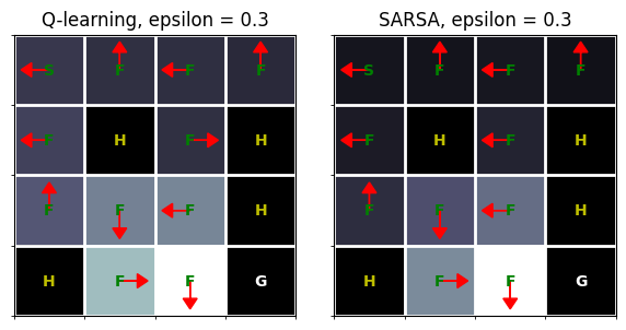
def td_control(seed, env, num_episodes, epsilon, on_policy):
    """Q-learning and SARSA in one loop: they differ in a single symbol."""
    rng = np.random.default_rng(seed)
    Q, visits = np.zeros((16, 4)), np.zeros((16, 4))
    env.reset(seed=seed)
    for _ in range(num_episodes):
        s, done = env.reset()[0], False
        a = d2l.epsilon_greedy(Q[s], epsilon, rng)
        while not done:
            s2, r, terminated, truncated, _ = env.step(a)
            a2 = d2l.epsilon_greedy(Q[s2], epsilon, rng)
            target = Q[s2, a2] if on_policy else Q[s2].max()  # the symbol
            visits[s, a] += 1
            Q[s, a] += (r + gamma * (1 - terminated) * target
                        - Q[s, a]) / (1 + 0.1 * visits[s, a])
            s, a, done = s2, a2, terminated or truncated
    return Q

Q_q = td_control(0, env, 8000, epsilon, on_policy=False)
Q_sarsa = td_control(0, env, 8000, epsilon, on_policy=True)
d2l.show_grid(env.unwrapped.desc, np.stack([Q_q.max(-1), Q_sarsa.max(-1)]),
              np.stack([Q_q.argmax(-1), Q_sarsa.argmax(-1)]),
              titles=['Q-learning, epsilon = 0.3', 'SARSA, epsilon = 0.3'])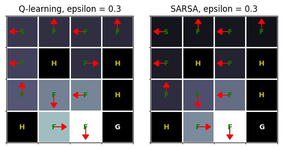
The greedy policies differ only at state \(6\), where the two symmetric actions have equal optimal value as discussed in Section 14.4. Their value tables nevertheless represent different quantities. Q-learning estimates \(0.182\) at the start, close to the optimal value \(V^*(s_0)=0.180\). SARSA’s largest start-state entry is \(0.062\) because its continuation includes \(\epsilon\)-greedy exploration, which sometimes moves toward a hole.
Since SARSA estimates \(Q^{\pi_e}\), its start-state value is not \(\max_a Q(s_0,a)\) but the policy-weighted average \(\sum_a\pi_e(a\mid s_0)Q(s_0,a)\). The following evaluation compares each table with the policy whose return it is intended to predict:
env.reset(seed=1)
rng = np.random.default_rng(1)
for name, Q in [('Q-learning', Q_q), ('SARSA', Q_sarsa)]:
    greedy = d2l.evaluate(env, lambda s, r_: int(Q[s].argmax()), 1000)
    earned = d2l.evaluate(env, lambda s, r_: d2l.epsilon_greedy(
        Q[s], epsilon, r_), 1000, gamma, rng)
    claim = (1 - epsilon) * Q[0].max() + epsilon * Q[0].mean()
    print(f'{name:>10}: greedy policy succeeds {greedy:.1%}; '
          f'the behavior earns {earned:.3f}')
    print(f'{"":>10}  the policy-weighted table value '
          f'sum_a pi(a|s0) Q(s0, a) claims {claim:.3f}')
Q-learning: greedy policy succeeds 72.5%; the behavior earns 0.061
the policy-weighted table value sum_a pi(a|s0) Q(s0, a) claims 0.180
SARSA: greedy policy succeeds 74.1%; the behavior earns 0.070
the policy-weighted table value sum_a pi(a|s0) Q(s0, a) claims 0.061env.reset(seed=1)
rng = np.random.default_rng(1)
for name, Q in [('Q-learning', Q_q), ('SARSA', Q_sarsa)]:
greedy = d2l.evaluate(env, lambda s, r_: int(Q[s].argmax()), 1000)
earned = d2l.evaluate(env, lambda s, r_: d2l.epsilon_greedy(
Q[s], epsilon, r_), 1000, gamma, rng)
claim = (1 - epsilon) * Q[0].max() + epsilon * Q[0].mean()
print(f'{name:>10}: greedy policy succeeds {greedy:.1%}; '
f'the behavior earns {earned:.3f}')
print(f'{"":>10} the policy-weighted table value '
f'sum_a pi(a|s0) Q(s0, a) claims {claim:.3f}')Q-learning: greedy policy succeeds 72.5%; the behavior earns 0.061
the policy-weighted table value sum_a pi(a|s0) Q(s0, a) claims 0.180
SARSA: greedy policy succeeds 74.1%; the behavior earns 0.070
the policy-weighted table value sum_a pi(a|s0) Q(s0, a) claims 0.061The two tables evaluate different policies. Q-learning assigns values to greedy continuation, even though the agent collected data with an \(\epsilon=0.3\) behavior policy. If its table is interpreted as the behavior policy’s value, it predicts \(0.180\) instead of the observed \(0.061\). SARSA accounts for the exploratory actions and predicts \(0.061\), within a hundredth of the observed \(0.070\). Their greedy policies both perform within a few percentage points of the \(73.6\) percent optimum from Section 14.2. The important difference is therefore the reference policy: Q-learning evaluates greedy continuation, whereas SARSA evaluates the behavior that generated the data. The latter is the relevant quantity when exploration remains part of deployment.
15.6.1.3 Bounded Staleness and Importance Ratios
The distinction is not absolute in practical systems. Importance ratios can correct data from a nearby policy, but their variance grows rapidly as the two policies separate; PPO therefore reuses each batch for only a limited number of epochs. In distributed learning, actors may also lag behind the central learner. IMPALA’s V-trace truncates importance corrections so that moderately stale data remains useful with controlled variance (Espeholt et al. 2018). The remainder of this section considers the extreme case: a fixed dataset with no further interaction.
15.6.2 Offline Learning
15.6.2.1 Measuring Distribution Shift
In offline reinforcement learning, a behavior policy collects a fixed dataset of transitions, and the learner receives no further interaction with the environment. It must choose a policy without exploring or testing its estimates through new actions. This setting, called batch reinforcement learning in older literature, arises when logged data are plentiful but experimentation is costly or unsafe, as with hospital records, driving logs, and the interaction history of a deployed system (Levine et al. 2020).
We continue with the slippery lake because its exact optimum is computable. We can therefore compare both predicted values and realized returns with the best achievable value, rather than with another learned method. The cited literature provides the corresponding deep-network experiments. Here the behavior policy selects actions uniformly at random:
def behavior(obs, rng):
    """The data-collection policy: uniformly random, no competence at all."""
    return int(rng.integers(4))

env.reset(seed=0)
data = d2l.rollout(env, behavior, num_episodes, np.random.default_rng(0))
counts = np.zeros((16, 4))
np.add.at(counts, (data.obs, data.act), 1)
live = np.isin(env.unwrapped.desc.flatten(), [b'S', b'F'])
print(f'{len(data)} transitions; support over the {4 * live.sum()} live '
      f'pairs: min {int(counts[live].min())}, median '
      f'{int(np.median(counts[live]))}, max {int(counts[live].max())}')
print(f'the behavior earned {data.episode_returns(gamma).mean():.3f} '
      f'per episode, discounted')
3997 transitions; support over the 44 live pairs: min 7, median 42, max 465
the behavior earned 0.012 per episode, discounteddef behavior(obs, rng):
"""The data-collection policy: uniformly random, no competence at all."""
return int(rng.integers(4))
env.reset(seed=0)
data = d2l.rollout(env, behavior, num_episodes, np.random.default_rng(0))
counts = np.zeros((16, 4))
np.add.at(counts, (data.obs, data.act), 1)
live = np.isin(env.unwrapped.desc.flatten(), [b'S', b'F'])
print(f'{len(data)} transitions; support over the {4 * live.sum()} live '
f'pairs: min {int(counts[live].min())}, median '
f'{int(np.median(counts[live]))}, max {int(counts[live].max())}')
print(f'the behavior earned {data.episode_returns(gamma).mean():.3f} '
f'per episode, discounted')3997 transitions; support over the 44 live pairs: min 7, median 42, max 465
the behavior earned 0.012 per episode, discountedThe 500 random episodes visit all \(44\) live state–action pairs, with at least \(7\) visits per pair and a median of \(42\). This coverage meets the tabular condition used in Section 14.4, but the behavior policy obtains only \(0.012\) return per episode, compared with the optimum of \(0.180\).
Broad coverage and poor behavior serve different purposes in the experiment. Coverage supplies information about every available action, while poor behavior leaves room for an offline learner to construct a better policy from those transitions.
Q-learning can use transitions from any behavior policy, so it can be applied to this fixed dataset: repeatedly shuffle the transitions, apply the usual updates, and stop when the values settle. However, outperforming the behavior policy requires counterfactual estimates for actions that appear rarely, or not at all, in the data. These estimates must be obtained by generalizing from observed actions (Levine et al. 2020).
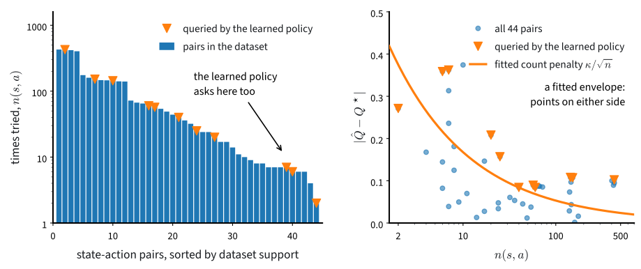
The learned policy preferentially selects actions with large estimated values. Estimation errors are largest where the dataset provides the least support, so this selection can concentrate the policy on poorly estimated actions. The resulting mismatch between the dataset’s action distribution and the learned policy’s action distribution is called distribution shift. In Figure 15.6.2, several actions selected by the learned policy lie in the sparsely sampled region where the fitted values have the largest errors.
15.6.2.2 The Loss of Self-Correction
Offline learning removes the self-correction available in Section 14.4. Online, an overestimated action is eventually selected, tested, and corrected by new data. Offline, the learned policy may select the same action repeatedly in evaluation, but the training dataset never changes and the estimate receives no corrective transition.
Maximization makes this problem systematic. A maximum over noisy estimates is biased upward, as Section 14.4 introduced and Figure 15.4.3 measures. The greedy policy selects the largest errors rather than typical errors, and bootstrapping propagates those inflated values to earlier states. The same optimization pressure appeared in Section 15.3, where a policy exploited errors in a learned reward. Here the errors occur in the value function and enter through the maximum in every backup.
15.6.2.3 The Experiment and the Behavior-Cloning Baseline
The experiment requires an offline algorithm, two comparison methods, and a known optimum. The function below repeatedly shuffles the fixed dataset and applies the Q-learning update. Its parameter kappa controls a pessimistic penalty developed in the next section; kappa = 0 gives naive offline Q-learning. An unobserved state–action pair has count \(n=0\) and must not be treated as though it had one observation. With pessimism enabled, such pairs receive the lowest possible value on this nonnegative-reward environment:
def offline_q(batch, num_sweeps, alpha, gamma, kappa=0.0,
              shape=(16, 4), seed=0):
    """Q-learning swept over a fixed dataset, with optional pessimism.

    kappa > 0 subtracts kappa/sqrt(n(s, a)) from every value consulted;
    an untried pair is distrusted entirely, and no pessimistic value
    drops below zero, the floor this environment guarantees.
    """
    Q, counts = np.zeros(shape), np.zeros(shape)
    np.add.at(counts, (batch.obs, batch.act), 1)
    penalty = np.where(counts > 0, kappa / np.sqrt(np.maximum(counts, 1)),
                       np.inf if kappa > 0 else 0.0)
    rng = np.random.default_rng(seed)
    for _ in range(num_sweeps):
        for i in rng.permutation(len(batch)):
            s, a, s2 = batch.obs[i], batch.act[i], batch.next_obs[i]
            v2 = np.maximum(Q[s2] - penalty[s2], 0.0).max()
            Q[s, a] += alpha * (batch.rew[i] + gamma
                                * (1 - batch.term[i]) * v2 - Q[s, a])
    return np.maximum(Q - penalty, 0.0)
def offline_q(batch, num_sweeps, alpha, gamma, kappa=0.0,
shape=(16, 4), seed=0):
"""Q-learning swept over a fixed dataset, with optional pessimism.
kappa > 0 subtracts kappa/sqrt(n(s, a)) from every value consulted;
an untried pair is distrusted entirely, and no pessimistic value
drops below zero, the floor this environment guarantees.
"""
Q, counts = np.zeros(shape), np.zeros(shape)
np.add.at(counts, (batch.obs, batch.act), 1)
penalty = np.where(counts > 0, kappa / np.sqrt(np.maximum(counts, 1)),
np.inf if kappa > 0 else 0.0)
rng = np.random.default_rng(seed)
for _ in range(num_sweeps):
for i in rng.permutation(len(batch)):
s, a, s2 = batch.obs[i], batch.act[i], batch.next_obs[i]
v2 = np.maximum(Q[s2] - penalty[s2], 0.0).max()
Q[s, a] += alpha * (batch.rew[i] + gamma
* (1 - batch.term[i]) * v2 - Q[s, a])
return np.maximum(Q - penalty, 0.0)The first comparison method is behavior cloning from Section 14.3, a standard baseline for offline learning. In the tabular setting, cross-entropy training recovers the empirical action distribution at each state, which can be computed by counting. Because the behavior policy is stochastic, the clone also samples its actions. Its predicted performance is the dataset’s average return.
def clone_policy(batch, num_actions=4):
    """Behavior cloning on a table: the dataset's empirical action
    distribution, uniform wherever the dataset is silent."""
    counts = np.zeros((16, num_actions))
    np.add.at(counts, (batch.obs, batch.act), 1)
    total = counts.sum(axis=1, keepdims=True)
    probs = np.where(total > 0, counts / np.maximum(total, 1), 1 / num_actions)
    return lambda s, rng: int(rng.choice(num_actions, p=probs[s]))
def clone_policy(batch, num_actions=4):
"""Behavior cloning on a table: the dataset's empirical action
distribution, uniform wherever the dataset is silent."""
counts = np.zeros((16, num_actions))
np.add.at(counts, (batch.obs, batch.act), 1)
total = counts.sum(axis=1, keepdims=True)
probs = np.where(total > 0, counts / np.maximum(total, 1), 1 / num_actions)
return lambda s, rng: int(rng.choice(num_actions, p=probs[s]))The environment model is available to the experimenter but not to the learning algorithms. Value iteration from Section 14.2 therefore supplies the exact value of the best possible policy:
V_star = d2l.value_iteration(mdp, num_iters=1000)[-1]
Q_star = mdp.backup(V_star)
print(f'the yardstick no offline deployment has: V*(s0) = {V_star[0]:.3f}')
the yardstick no offline deployment has: V*(s0) = 0.180V_star = d2l.value_iteration(mdp, num_iters=1000)[-1]
Q_star = mdp.backup(V_star)
print(f'the yardstick no offline deployment has: V*(s0) = {V_star[0]:.3f}')the yardstick no offline deployment has: V*(s0) = 0.180We repeat the experiment on fifteen independently collected datasets because results from one set of 500 random episodes vary substantially. On each dataset, we train naive offline Q-learning, its pessimistic variant, and behavior cloning. For every method, we record the predicted start-state value and the return obtained by its learned policy:
datasets, fits = [], []
results = {name: ([], []) for name in ['naive', 'pessimistic', 'clone']}
for seed in range(num_datasets):
    env.reset(seed=seed)
    rng = np.random.default_rng(seed)
    batch = d2l.rollout(env, behavior, num_episodes, rng)
    datasets.append(batch)
    Q_n = offline_q(batch, num_sweeps, alpha, gamma)
    fits.append(Q_n)
    for name, Q in [('naive', Q_n), ('pessimistic', offline_q(
            batch, num_sweeps, alpha, gamma, kappa))]:
        results[name][0].append(Q[0].max())
        results[name][1].append(d2l.evaluate(
            env, lambda s, r_: int(Q[s].argmax()), 500, gamma, rng))
    results['clone'][0].append(batch.episode_returns(gamma).mean())
    results['clone'][1].append(d2l.evaluate(env, clone_policy(batch),
                                            500, gamma, rng))
datasets, fits = [], []
results = {name: ([], []) for name in ['naive', 'pessimistic', 'clone']}
for seed in range(num_datasets):
env.reset(seed=seed)
rng = np.random.default_rng(seed)
batch = d2l.rollout(env, behavior, num_episodes, rng)
datasets.append(batch)
Q_n = offline_q(batch, num_sweeps, alpha, gamma)
fits.append(Q_n)
for name, Q in [('naive', Q_n), ('pessimistic', offline_q(
batch, num_sweeps, alpha, gamma, kappa))]:
results[name][0].append(Q[0].max())
results[name][1].append(d2l.evaluate(
env, lambda s, r_: int(Q[s].argmax()), 500, gamma, rng))
results['clone'][0].append(batch.episode_returns(gamma).mean())
results['clone'][1].append(d2l.evaluate(env, clone_policy(batch),
500, gamma, rng))for name, (pred, actual) in results.items():
print(f'{name:>11}: predicted median {np.median(pred):.3f}, '
f'spread {min(pred):.3f} to {max(pred):.3f}')
print(f'{"":>11} actual median {np.median(actual):.3f}, '
f'spread {min(actual):.3f} to {max(actual):.3f}')
over = [sum(p > V_star[0] for p in results[k][0])
for k in ['naive', 'pessimistic']]
print(f'promises above V*(s0): naive on {over[0]} of {num_datasets} '
f'datasets, pessimistic on {over[1]} of {num_datasets}')
wins = sum(p > q for p, q in zip(results['pessimistic'][1],
results['naive'][1]))
print(f'pessimism delivered the better policy on {wins} of '
f'{num_datasets} datasets') naive: predicted median 0.274, spread 0.185 to 0.388
actual median 0.097, spread 0.070 to 0.184
pessimistic: predicted median 0.121, spread 0.035 to 0.225
actual median 0.080, spread 0.050 to 0.189
clone: predicted median 0.007, spread 0.004 to 0.014
actual median 0.008, spread 0.003 to 0.014
promises above V*(s0): naive on 15 of 15 datasets, pessimistic on 2 of 15
pessimism delivered the better policy on 4 of 15 datasetsfor name, (pred, actual) in results.items():
print(f'{name:>11}: predicted median {np.median(pred):.3f}, '
f'spread {min(pred):.3f} to {max(pred):.3f}')
print(f'{"":>11} actual median {np.median(actual):.3f}, '
f'spread {min(actual):.3f} to {max(actual):.3f}')
over = [sum(p > V_star[0] for p in results[k][0])
for k in ['naive', 'pessimistic']]
print(f'promises above V*(s0): naive on {over[0]} of {num_datasets} '
f'datasets, pessimistic on {over[1]} of {num_datasets}')
wins = sum(p > q for p, q in zip(results['pessimistic'][1],
results['naive'][1]))
print(f'pessimism delivered the better policy on {wins} of '
f'{num_datasets} datasets') naive: predicted median 0.274, spread 0.185 to 0.388
actual median 0.097, spread 0.070 to 0.184
pessimistic: predicted median 0.121, spread 0.035 to 0.225
actual median 0.080, spread 0.050 to 0.189
clone: predicted median 0.007, spread 0.004 to 0.014
actual median 0.008, spread 0.003 to 0.014
promises above V*(s0): naive on 15 of 15 datasets, pessimistic on 2 of 15
pessimism delivered the better policy on 4 of 15 datasetsnames = list(results)
x, w = np.arange(len(names)), 0.35
d2l.set_figsize((5.5, 3.5))
for i, side in enumerate(['predicted value at the start', 'actual return']):
vals = np.array([results[k][i] for k in names])
med = np.median(vals, axis=1)
d2l.plt.bar(x + w * i, med, w, label=side,
yerr=[med - vals.min(axis=1), vals.max(axis=1) - med],
capsize=3)
d2l.plt.axhline(V_star[0], ls='--', color='gray')
d2l.plt.xticks(x + w / 2, names)
d2l.plt.ylabel('discounted value')
d2l.plt.legend();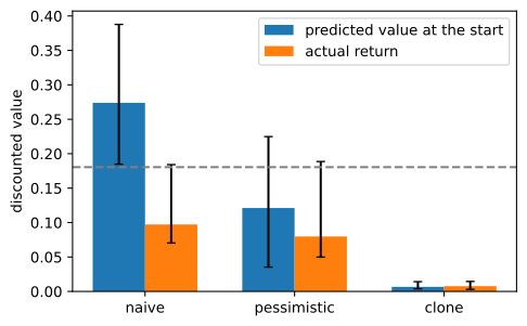
names = list(results)
x, w = np.arange(len(names)), 0.35
d2l.set_figsize((5.5, 3.5))
for i, side in enumerate(['predicted value at the start', 'actual return']):
    vals = np.array([results[k][i] for k in names])
    med = np.median(vals, axis=1)
    d2l.plt.bar(x + w * i, med, w, label=side,
                yerr=[med - vals.min(axis=1), vals.max(axis=1) - med],
                capsize=3)
d2l.plt.axhline(V_star[0], ls='--', color='gray')
d2l.plt.xticks(x + w / 2, names)
d2l.plt.ylabel('discounted value')
d2l.plt.legend();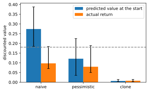
Across the fifteen datasets, naive offline Q-learning predicts a start-state value between \(0.185\) and \(0.388\), with median \(0.274\). The true optimum is \(0.180\), so every prediction exceeds the value achievable by any policy in this environment. Yet the learned greedy policies have a median return of only \(0.097\). Comparing predicted value with realized return is a standard diagnostic in offline reinforcement learning; with deep networks and continuous actions, the discrepancy can be much larger (Levine et al. 2020; Fujimoto et al. 2019).
Behavior cloning predicts a median value of \(0.007\) and obtains \(0.008\). It is well calibrated but reproduces the poor random behavior. Naive offline Q-learning produces policies with returns roughly an order of magnitude larger, even though it substantially overestimates their values.
These two comparisons measure different properties. Comparison with behavior cloning asks whether offline learning improves on the data-collection policy. Comparison of predicted and realized return asks whether its value estimates are calibrated. Naive Q-learning succeeds on the first criterion and fails on the second.
15.6.3 Pessimism
15.6.3.1 The Count-Based Penalty \(\kappa/\sqrt{n}\)
The largest errors occur at poorly supported state–action pairs. We therefore subtract \(\kappa/\sqrt{n(s,a)}\) both inside the bootstrap maximum and from the final values, where \(n(s,a)\) is the pair’s count in the dataset. This is the penalty implemented by offline_q when kappa > 0.
The \(1/\sqrt{n}\) dependence is motivated by the sampling error of an \(n\)-sample average and resembles the UCB radius \(\kappa\sqrt{\log t/n}\) from Section 14.4. Here it is a heuristic shrinkage term, not a confidence interval with a coverage guarantee. We evaluate this shape by pooling the counts and errors against \(Q^*\) from the fifteen naive runs:
support, error = [], []
for batch, Q in zip(datasets, fits):
    c = np.zeros((16, 4))
    np.add.at(c, (batch.obs, batch.act), 1)
    support.append(c[live].ravel())
    error.append(np.abs(Q - Q_star)[live].ravel())
support, error = np.concatenate(support), np.concatenate(error)
n, e = support[support > 0], error[support > 0]
kappa_fit = np.median(e * np.sqrt(n))
print(f'{len(n)} supported live pairs over {num_datasets} datasets: error '
      f'min {e.min():.3f}, median {np.median(e):.3f}, max {e.max():.3f}')
print(f'kappa centering kappa/sqrt(n) on the cloud: {kappa_fit:.2f}')
print(f'residual error at n > 100: median {np.median(e[n > 100]):.3f}')
grid = np.logspace(np.log10(n.min()), np.log10(n.max()), 50)
d2l.plot([n, grid], [e, kappa_fit / np.sqrt(grid)],
         xlabel='n(s, a) in the dataset', ylabel='error of the fitted value',
         legend=['one pair, one dataset', 'kappa/sqrt(n)'],
         xscale='log', fmts=('o', '-'), figsize=(5, 3.5))
659 supported live pairs over 15 datasets: error min 0.000, median 0.094, max 0.458
kappa centering kappa/sqrt(n) on the cloud: 0.57
residual error at n > 100: median 0.077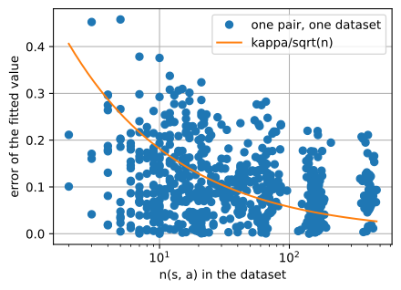
support, error = [], []
for batch, Q in zip(datasets, fits):
    c = np.zeros((16, 4))
    np.add.at(c, (batch.obs, batch.act), 1)
    support.append(c[live].ravel())
    error.append(np.abs(Q - Q_star)[live].ravel())
support, error = np.concatenate(support), np.concatenate(error)
n, e = support[support > 0], error[support > 0]
kappa_fit = np.median(e * np.sqrt(n))
print(f'{len(n)} supported live pairs over {num_datasets} datasets: error '
      f'min {e.min():.3f}, median {np.median(e):.3f}, max {e.max():.3f}')
print(f'kappa centering kappa/sqrt(n) on the cloud: {kappa_fit:.2f}')
print(f'residual error at n > 100: median {np.median(e[n > 100]):.3f}')
grid = np.logspace(np.log10(n.min()), np.log10(n.max()), 50)
d2l.plot([n, grid], [e, kappa_fit / np.sqrt(grid)],
         xlabel='n(s, a) in the dataset', ylabel='error of the fitted value',
         legend=['one pair, one dataset', 'kappa/sqrt(n)'],
         xscale='log', fmts=('o', '-'), figsize=(5, 3.5))
659 supported live pairs over 15 datasets: error min 0.000, median 0.094, max 0.458
kappa centering kappa/sqrt(n) on the cloud: 0.57
residual error at n > 100: median 0.077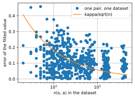
The fitted scale is \(\kappa=0.57\), but it only centers the curve on these fifteen datasets. The errors range from \(0.000\) to \(0.458\), with median \(0.094\), and do not follow a clean \(1/\sqrt{n}\) law. Even above 100 visits, their median remains \(0.077\). Maximization bias, the constant step size \(\alpha\), and incomplete convergence can all produce this residual, which additional samples do not necessarily remove.
Among the 660 state–action-pair and dataset combinations, one pair is unobserved and receives the \(n=0\) treatment defined above. We use the milder value \(\kappa=0.1\), about one fifth of the descriptive fit. Exercise 4 explores both smaller and larger penalties.
The example combines four distinct difficulties. Support failure occurs when an action or region is absent from the data. Statistical uncertainty remains when counts are finite and is the component approximated by \(1/\sqrt{n}\). Bootstrapped extrapolation propagates errors through function approximation and is largely absent from this tabular experiment. Finally, model selection requires choosing \(\kappa\) without the online evaluation that the setting forbids.
15.6.3.2 Optimism Online, Pessimism Offline
Online exploration and offline learning use similar count-dependent terms with opposite signs. UCB adds \(\kappa\sqrt{\log t/n}\) to favor actions with little data, whereas offline pessimism subtracts \(\kappa/\sqrt{n}\) to avoid relying on them. These terms express the same qualitative dependence on support but are not the same statistical quantity: the online bonus includes \(\log t\), and the two methods tune their scales for different objectives.
The difference follows from feedback. Online, an optimistic action can be selected and its estimate corrected with new observations; optimism can therefore drive exploration. Offline, no new observation can correct an optimistic error, so uncertainty is handled conservatively.
15.6.3.3 Calibration after Pessimism
The pessimistic estimate has median \(0.121\), down from \(0.274\), and exceeds the true optimum on only two of the fifteen datasets. Its range is \(0.035\) to \(0.225\). The policy itself is not better: it outperforms the naive policy on only four datasets, and its median return is \(0.080\) rather than \(0.097\). Pessimism has instead reduced the discrepancy between predicted and realized performance. More sophisticated versions of this conservative principle are common in modern offline reinforcement learning (Levine et al. 2020).
15.6.4 Beyond the Gridworld
15.6.4.1 Constraining the Policy, the Values, or Both
Exact counts are unavailable in continuous state and action spaces, but deep offline methods retain the same two responses: constrain the policy to supported actions or reduce values outside the data distribution. Batch-constrained Q-learning takes the first approach and restricts the learned policy to actions represented in the dataset (Fujimoto et al. 2019). Its tabular analogue replaces the graded penalty in offline_q with a hard support constraint:
def support_q(batch, num_sweeps, alpha, gamma, seed=0):
    """offline_q with the graded penalty replaced by a hard support rule."""
    Q, counts = np.zeros((16, 4)), np.zeros((16, 4))
    np.add.at(counts, (batch.obs, batch.act), 1)
    rng = np.random.default_rng(seed)
    for _ in range(num_sweeps):
        for i in rng.permutation(len(batch)):
            s, a, s2 = batch.obs[i], batch.act[i], batch.next_obs[i]
            v2 = np.where(counts[s2] > 0, Q[s2], 0.0).max()   # changed line 1
            Q[s, a] += alpha * (batch.rew[i] + gamma
                                * (1 - batch.term[i]) * v2 - Q[s, a])
    return np.where(counts > 0, Q, 0.0)                       # changed line 2

assert np.array_equal(support_q(data, num_sweeps, alpha, gamma), fits[0])
print('on this dataset the support rule reproduces the naive run, '
      'bit for bit')
on this dataset the support rule reproduces the naive run, bit for bitdef support_q(batch, num_sweeps, alpha, gamma, seed=0):
"""offline_q with the graded penalty replaced by a hard support rule."""
Q, counts = np.zeros((16, 4)), np.zeros((16, 4))
np.add.at(counts, (batch.obs, batch.act), 1)
rng = np.random.default_rng(seed)
for _ in range(num_sweeps):
for i in rng.permutation(len(batch)):
s, a, s2 = batch.obs[i], batch.act[i], batch.next_obs[i]
v2 = np.where(counts[s2] > 0, Q[s2], 0.0).max() # changed line 1
Q[s, a] += alpha * (batch.rew[i] + gamma
* (1 - batch.term[i]) * v2 - Q[s, a])
return np.where(counts > 0, Q, 0.0) # changed line 2
assert np.array_equal(support_q(data, num_sweeps, alpha, gamma), fits[0])
print('on this dataset the support rule reproduces the naive run, '
'bit for bit')on this dataset the support rule reproduces the naive run, bit for bitOn this dataset, the hard support constraint reproduces naive Q-learning exactly. Values start at zero, rewards are nonnegative, and every available pair has at least seven observations. An unobserved action therefore cannot obtain a larger value than an observed one, and no available action is actually unobserved. The failure here is variation in the amount of support, which a binary rule cannot distinguish but \(\kappa/\sqrt{n}\) can.
In continuous action spaces, almost every exact action is absent from the dataset, so support constraints become more important. Conservative Q-learning instead penalizes the values of out-of-distribution actions (Kumar et al. 2020). Implicit Q-learning avoids querying unseen actions by backing up an upper expectile of values observed in the dataset (Kostrikov et al. 2022). TD3+BC adds a behavior-cloning term to an off-policy actor and provides a strong simple baseline (Fujimoto and Gu 2021).
Most practical offline methods constrain the policy, the value estimates, or both.
15.6.4.2 Sequence Modeling without Bootstrapping
Decision Transformer avoids bootstrapping by treating each trajectory as a sequence of returns-to-go, states, and actions (Chen et al. 2021). An autoregressive model is trained by supervised prediction and, at test time, is conditioned on a desired return. It uses neither a value function nor a maximization target. On standard benchmarks, this approach matches strong value-based offline methods. However, a later study found that a small return-conditioned network trained by ordinary supervised learning recovers much of the performance, so the contribution of the sequence architecture remains unsettled. Section 15.7 returns to this connection for language models.
15.6.4.3 Offline Model Selection
The preceding comparisons use simulator rollouts, which are unavailable in a genuine offline deployment. Selecting \(\kappa\), the number of sweeps, or one of several learned policies requires estimating counterfactual performance from logged data. Importance-weighted estimators for this task inherit the high variance described in Section 15.2 when the evaluated policy differs from the behavior policy (Levine et al. 2020).
Reliable offline model selection remains an open problem. Exercise 6 examines what can be inferred when direct evaluation rollouts are unavailable.
15.6.5 Summary
On-policy updates estimate expectations under the current policy; importance ratios permit limited correction for older policies. Q-learning is off-policy because its Bellman target does not depend on the data-collection policy, whereas SARSA evaluates the behavior policy itself. Offline reinforcement learning applies off-policy updates to a fixed dataset. Without interaction, overestimated actions outside the dataset’s support cannot be tested and corrected. A count-based pessimistic penalty reduces these estimates but does not guarantee a better policy. Deep offline methods likewise constrain policies, values, or both, and model selection without online evaluation remains difficult.
Experimental scope. The SARSA comparison uses one seed and one exploration rate. The offline experiment reports fifteen independently collected datasets and 500 evaluation episodes per learned policy. Naive offline Q-learning predicts values above the known optimum on every dataset. Pessimism substantially improves calibration but does not improve median return in this example. Exact optimal values are available only because the experiment uses a small known MDP.
15.6.6 Exercises
- [short-code] Does the clone win? Add a behavior-cloning arm on each of the three dataset types of exercise 3 and report which arm wins on each; explain the pattern in terms of the behavior policy’s quality.
- [short-code] More data, or better data. Rerun the offline experiment with datasets of 100, 500 and 2000 episodes. How do the predicted and the actual values move? Does more random data close the gap by itself, and if not, what is it that more data does not buy?
- [short-code] Where the data comes from. Build three datasets of 500 episodes each: from a uniform random policy, from a near-optimal policy with \(\epsilon = 0.1\), and from a fifty-fifty mixture. Run naive offline Q-learning on each and report predicted value and actual return. Which dataset yields the best policy, which the best-calibrated prediction, and why is the expert-only dataset not the winner?
- [short-code] How much pessimism. Sweep \(\kappa\) over \(\{0.02, 0.1, 0.3, 1.0\}\). Describe both failure directions: what happens when pessimism is too weak, and what happens when it is too strong? Plot predicted value and actual return on the same axes and identify the crossing.
- [conceptual] Constrain the values, or constrain the policy. The text’s support rule reproduced the naive run exactly, and the argument for why leaned on zero initialization and nonnegative rewards. Construct a behavior policy, or an initialization, for which the support rule and the count penalty genuinely differ, and say which of the two you would trust with a dataset gathered by a safety-conscious human operator.
- [conceptual] What you cannot measure offline. Our diagnostic compared the predicted value with the actual return of the greedy policy, which required rolling the policy out in the simulator. A real offline deployment cannot do that. Name what you would use instead, say what each of those estimators needs that our setting supplies for free, and explain why the whole family inherits a version of the variance problem of Section 15.2.