from d2l import torch as d2l
import logging
# Use INFO level so the periodic Syne Tune tuning-status table appears,
# but use a clean format that drops the "INFO:syne_tune.tuner:" prefix.
logging.basicConfig(level=logging.INFO, format="%(message)s", force=True)
import matplotlib.pyplot as plt
# Silence Syne Tune's import-time chatter about optional AWS dependencies
# (sagemaker, s3fs) and Ray Tune. We use the local PythonBackend, so those
# are not needed. Suppress both print() and logging.info() during imports.
import contextlib, io
_root = logging.getLogger()
_prev_level = _root.level
_root.setLevel(logging.WARNING)
try:
    with contextlib.redirect_stdout(io.StringIO()):
        from syne_tune.config_space import loguniform, randint
        from syne_tune.backend.python_backend.python_backend import PythonBackend
        from syne_tune.optimizer.baselines import ASHA
        from syne_tune import Tuner, StoppingCriterion
        from syne_tune.experiments import load_experiment
finally:
    _root.setLevel(_prev_level)

# Silence the per-trial subprocess-command spam from local_backend and
# drop the per-trial scheduling / completion lines from the tuner logger.
# Keep the periodic "tuning status (last metric is reported)" updates so
# the reader can still see progress over time.
class _DropPerTrialNoise(logging.Filter):
    _DROP = (
        "results of trials will be saved",
        "scheduled ",
        "Trial trial_id ",
    )
    def filter(self, record):
        msg = record.getMessage()
        return not any(s in msg for s in self._DROP)

logging.getLogger("syne_tune.backend.local_backend").setLevel(logging.WARNING)
logging.getLogger("syne_tune.tuner").addFilter(_DropPerTrialNoise())22.5 Asynchronous Successive Halving
As we have seen in Section 22.3, we can accelerate HPO by distributing the evaluation of hyperparameter configurations across either multiple instances or multiple CPUs / GPUs on a single instance. However, compared to random search, it is not straightforward to run successive halving (SH) asynchronously in a distributed setting. Before we can decide which configuration to run next, we first have to collect all observations at the current rung level. This requires to synchronize workers at each rung level. For example, for the lowest rung level \(r_{\mathrm{min}}\), we first have to evaluate all \(N = \eta^K\) configurations, before we can promote the \(\frac{1}{\eta}\) of them to the next rung level.
In any distributed system, synchronization typically implies idle time for workers. First, we often observe high variations in training time across hyperparameter configurations. For example, assuming the number of filters per layer is a hyperparameter, then networks with less filters finish training faster than networks with more filters, which implies idle worker time due to stragglers. Moreover, the number of slots in a rung level is not always a multiple of the number of workers, in which case some workers may even sit idle for a full batch.
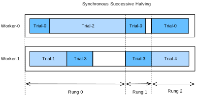
Figure Figure 22.5.1 shows the scheduling of synchronous SH with \(\eta=2\) for four different trials with two workers. We start with evaluating Trial-0 and Trial-1 for one epoch and immediately continue with the next two trials once they are finished. We first have to wait until Trial-2 finishes, which takes substantially more time than the other trials, before we can promote the best two trials, i.e., Trial-0 and Trial-3 to the next rung level. This causes idle time for Worker-1. Then, we continue with Rung 1. Also, here Trial-3 takes longer than Trial-0, which leads to an additional idling time of Worker-0. Once we reach Rung-2, only the best trial, Trial-0, remains which occupies only one worker. To avoid that Worker-1 idles during that time, most implementations of SH continue already with the next round, and start evaluating new trials (e.g Trial-4) on the first rung.
Asynchronous successive halving (ASHA) (Li et al. 2018) adapts SH to the asynchronous parallel scenario. The main idea of ASHA is to promote configurations to the next rung level as soon as we collected at least \(\eta\) observations on the current rung level. This decision rule may lead to suboptimal promotions: configurations can be promoted to the next rung level, which in hindsight do not compare favourably against most others at the same rung level. On the other hand, we get rid of all synchronization points this way. In practice, such suboptimal initial promotions have only a modest impact on performance, not only because the ranking of hyperparameter configurations is often fairly consistent across rung levels, but also because rungs grow over time and reflect the distribution of metric values at this level better and better. If a worker is free, but no configuration can be promoted, we start a new configuration with \(r = r_{\mathrm{min}}\), i.e the first rung level.
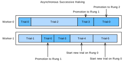
Figure 22.5.2 shows the scheduling of the same configurations for ASHA. Once Trial-1 finishes, we collect the results of two trials (i.e Trial-0 and Trial-1) and immediately promote the better of them (Trial-0) to the next rung level. After Trial-0 finishes on rung 1, there are too few trials there in order to support a further promotion. Hence, we continue with rung 0 and evaluate Trial-3. Once Trial-3 finishes, Trial-2 is still pending. At this point we have 3 trials evaluated on rung 0 and one trial evaluated already on rung 1. Since Trial-3 performs worse than Trial-0 at rung 0, and \(\eta=2\), we cannot promote any new trial yet, and Worker-1 starts Trial-4 from scratch instead. However, once Trial-2 finishes and scores worse than Trial-3, the latter is promoted towards rung 1. Afterwards, we collected 2 evaluations on rung 1, which means we can now promote Trial-0 towards rung 2. At the same time, Worker-1 continues with evaluating new trials (i.e., Trial-5) on rung 0.
22.5.1 Objective Function
We will use Syne Tune with the same objective function as in Section 22.3.
def hpo_objective_lenet_synetune(learning_rate, batch_size, max_epochs):
    from d2l import torch as d2l
    from syne_tune import Reporter

    model = d2l.LeNet(lr=learning_rate, num_classes=10)
    trainer = d2l.HPOTrainer(max_epochs=1, num_gpus=1)
    data = d2l.FashionMNIST(batch_size=batch_size)
    model.apply_init([next(iter(data.get_dataloader(True)))[0]], d2l.init_cnn)
    report = Reporter()
    for epoch in range(1, max_epochs + 1):
        if epoch == 1:
            # Initialize the state of Trainer
            trainer.fit(model=model, data=data)
        else:
            trainer.fit_epoch()
        validation_error = d2l.numpy(trainer.validation_error().cpu())
        report(epoch=epoch, validation_error=float(validation_error))
We will also use the same configuration space as before:
min_number_of_epochs = 2
max_number_of_epochs = 10
eta = 2

config_space = {
    "learning_rate": loguniform(1e-2, 1),
    "batch_size": randint(32, 256),
    "max_epochs": max_number_of_epochs,
}
initial_config = {
    "learning_rate": 0.1,
    "batch_size": 128,
}
22.5.2 Asynchronous Scheduler
First, we define the number of workers that evaluate trials concurrently. We also need to specify how long we want to run random search, by defining an upper limit on the total wall-clock time.
# Each LeNet trial fits in well under 7 GB of GPU memory, so we can pack
# multiple trials per device. `PythonBackend(rotate_gpus=True)` (the
# default) round-robins trials across detected GPUs and falls back to
# sharing when `n_workers > num_gpus`. Allocate 7 GB per slot — this
# yields 3 slots on a 24 GB card and 4 slots on a 32 GB card after
# driver overhead, e.g. 4×24 GB → 12 slots; 2×32 GB → 8.
import torch
_GB = 1024 ** 3
n_workers = sum(
    torch.cuda.get_device_properties(i).total_memory // (7 * _GB)
    for i in range(torch.cuda.device_count())
) or 1
max_wallclock_time = 15 * 60  # 15 minutes
The code for running ASHA is a simple variation of what we did for asynchronous random search.
mode = "min"
metric = "validation_error"
resource_attr = "epoch"

scheduler = ASHA(
    config_space,
    metric=metric,
    mode=mode,
    points_to_evaluate=[initial_config],
    max_resource_attr="max_epochs",
    resource_attr=resource_attr,
    grace_period=min_number_of_epochs,
    reduction_factor=eta,
)
max_resource_level = 10, as inferred from config_space
Master random_seed = 500938081Here, metric and resource_attr specify the key names used with the report callback, and max_resource_attr denotes which input to the objective function corresponds to \(r_{\mathrm{max}}\). Moreover, grace_period provides \(r_{\mathrm{min}}\), and reduction_factor is \(\eta\). We can run Syne Tune as before (this will take about 15 minutes):
trial_backend = PythonBackend(
    tune_function=hpo_objective_lenet_synetune,
    config_space=config_space,
)

stop_criterion = StoppingCriterion(max_wallclock_time=max_wallclock_time)
tuner = Tuner(
    trial_backend=trial_backend,
    scheduler=scheduler,
    stop_criterion=stop_criterion,
    n_workers=n_workers,
    print_update_interval=int(max_wallclock_time * 0.6),
)
tuner.run()
tuning status (last metric is reported)
trial_id status iter learning_rate batch_size max_epochs epoch validation_error worker-time
0 Completed 10 0.100000 128 10 10.0 0.259593 41.986538
1 Stopped 8 0.056396 78 10 8.0 0.296909 61.573820
2 Completed 10 0.146175 59 10 10.0 0.182669 71.431907
3 Completed 10 0.264778 64 10 10.0 0.177349 53.496369
4 Stopped 2 0.121276 131 10 2.0 0.899686 8.651651
5 Stopped 2 0.027298 186 10 2.0 0.900068 7.160189
6 Stopped 4 0.111784 192 10 4.0 0.891509 14.651674
7 Stopped 2 0.081205 160 10 2.0 0.899802 7.330440
8 Stopped 4 0.016171 49 10 4.0 0.898208 50.229704
9 Stopped 2 0.018324 94 10 2.0 0.899936 9.223270
10 Stopped 4 0.131451 131 10 4.0 0.630848 19.747981
11 Completed 10 0.169869 42 10 10.0 0.192668 72.582492
12 Completed 10 0.457482 126 10 10.0 0.198551 36.484710
13 Stopped 2 0.011669 247 10 2.0 0.899791 7.745016
14 Completed 10 0.354470 218 10 10.0 0.250189 42.595854
15 Completed 10 0.771696 175 10 10.0 0.170148 33.222969
16 Stopped 3 0.078584 210 10 3.0 0.899878 9.981106
17 Stopped 2 0.010755 207 10 2.0 0.900529 8.279234
18 Completed 10 0.158359 74 10 10.0 0.200457 46.442791
19 Stopped 2 0.085902 143 10 2.0 0.899980 12.516283
20 Stopped 3 0.253785 233 10 3.0 0.735960 10.463591
21 Stopped 2 0.089063 82 10 2.0 0.900009 15.709679
22 Stopped 2 0.030989 164 10 2.0 0.900000 8.351473
23 Stopped 4 0.050168 144 10 4.0 0.890625 13.669940
24 Stopped 2 0.026944 47 10 2.0 0.900018 25.221657
25 Stopped 2 0.022586 117 10 2.0 0.900280 7.875754
26 Stopped 2 0.034740 87 10 2.0 0.900013 8.801667
27 Stopped 3 0.067225 253 10 3.0 0.900205 9.223531
28 Stopped 3 0.064993 177 10 3.0 0.900080 10.073560
29 Stopped 3 0.040365 170 10 3.0 0.899979 10.254585
30 Completed 10 0.985882 142 10 10.0 0.157720 34.224341
31 Completed 10 0.853338 160 10 10.0 0.156051 33.598172
32 Stopped 3 0.122215 152 10 3.0 0.900133 10.413571
33 Completed 10 0.421837 109 10 10.0 0.181043 36.945569
34 Completed 10 0.848521 51 10 10.0 0.137950 59.422441
35 Completed 10 0.511322 194 10 10.0 0.192929 31.153330
36 Stopped 4 0.163844 191 10 4.0 0.599363 12.762001
37 Stopped 2 0.040626 47 10 2.0 0.900049 13.280510
38 Stopped 3 0.146771 241 10 3.0 0.842590 9.556640
39 Stopped 4 0.013122 212 10 4.0 0.901249 13.311442
40 Stopped 4 0.987861 167 10 4.0 0.299173 13.325593
41 Stopped 4 0.062355 185 10 4.0 0.901720 12.845736
42 Completed 10 0.543335 90 10 10.0 0.155357 41.359770
43 Stopped 3 0.087332 192 10 3.0 0.900649 9.801860
44 Stopped 5 0.224684 252 10 5.0 0.378793 14.790177
45 Stopped 10 0.787317 53 10 10.0 0.157762 55.888806
46 Completed 10 0.736108 171 10 10.0 0.181133 32.239157
47 InProgress 6 0.548450 33 10 6.0 0.154308 49.858660
48 Stopped 2 0.029855 51 10 2.0 0.900468 11.212459
49 Stopped 5 0.177382 222 10 5.0 0.400725 15.563592
50 Stopped 3 0.040421 206 10 3.0 0.900432 9.479672
51 InProgress 1 0.017261 86 10 1.0 0.900359 4.599208
52 InProgress 0 0.317794 53 10 - - -
3 trials running, 50 finished (15 until the end), 541.99s wallclock-time
reaching max wallclock time (900), stopping there.
Stopping trials that may still be running.
Tuning finished, results of trials can be found on syne-tune/python-entrypoint-2026-07-28-18-03-03-534--------------------
Resource summary (last result is reported):
trial_id status iter learning_rate batch_size max_epochs epoch validation_error worker-time
0 Completed 10 0.100000 128 10 10.0 0.259593 41.986538
1 Stopped 8 0.056396 78 10 8.0 0.296909 61.573820
2 Completed 10 0.146175 59 10 10.0 0.182669 71.431907
3 Completed 10 0.264778 64 10 10.0 0.177349 53.496369
4 Stopped 2 0.121276 131 10 2.0 0.899686 8.651651
5 Stopped 2 0.027298 186 10 2.0 0.900068 7.160189
6 Stopped 4 0.111784 192 10 4.0 0.891509 14.651674
7 Stopped 2 0.081205 160 10 2.0 0.899802 7.330440
8 Stopped 4 0.016171 49 10 4.0 0.898208 50.229704
9 Stopped 2 0.018324 94 10 2.0 0.899936 9.223270
10 Stopped 4 0.131451 131 10 4.0 0.630848 19.747981
11 Completed 10 0.169869 42 10 10.0 0.192668 72.582492
12 Completed 10 0.457482 126 10 10.0 0.198551 36.484710
13 Stopped 2 0.011669 247 10 2.0 0.899791 7.745016
14 Completed 10 0.354470 218 10 10.0 0.250189 42.595854
15 Completed 10 0.771696 175 10 10.0 0.170148 33.222969
16 Stopped 3 0.078584 210 10 3.0 0.899878 9.981106
17 Stopped 2 0.010755 207 10 2.0 0.900529 8.279234
18 Completed 10 0.158359 74 10 10.0 0.200457 46.442791
19 Stopped 2 0.085902 143 10 2.0 0.899980 12.516283
20 Stopped 3 0.253785 233 10 3.0 0.735960 10.463591
21 Stopped 2 0.089063 82 10 2.0 0.900009 15.709679
22 Stopped 2 0.030989 164 10 2.0 0.900000 8.351473
23 Stopped 4 0.050168 144 10 4.0 0.890625 13.669940
24 Stopped 2 0.026944 47 10 2.0 0.900018 25.221657
25 Stopped 2 0.022586 117 10 2.0 0.900280 7.875754
26 Stopped 2 0.034740 87 10 2.0 0.900013 8.801667
27 Stopped 3 0.067225 253 10 3.0 0.900205 9.223531
28 Stopped 3 0.064993 177 10 3.0 0.900080 10.073560
29 Stopped 3 0.040365 170 10 3.0 0.899979 10.254585
30 Completed 10 0.985882 142 10 10.0 0.157720 34.224341
31 Completed 10 0.853338 160 10 10.0 0.156051 33.598172
32 Stopped 3 0.122215 152 10 3.0 0.900133 10.413571
33 Completed 10 0.421837 109 10 10.0 0.181043 36.945569
34 Completed 10 0.848521 51 10 10.0 0.137950 59.422441
35 Completed 10 0.511322 194 10 10.0 0.192929 31.153330
36 Stopped 4 0.163844 191 10 4.0 0.599363 12.762001
37 Stopped 2 0.040626 47 10 2.0 0.900049 13.280510
38 Stopped 3 0.146771 241 10 3.0 0.842590 9.556640
39 Stopped 4 0.013122 212 10 4.0 0.901249 13.311442
40 Stopped 4 0.987861 167 10 4.0 0.299173 13.325593
41 Stopped 4 0.062355 185 10 4.0 0.901720 12.845736
42 Completed 10 0.543335 90 10 10.0 0.155357 41.359770
43 Stopped 3 0.087332 192 10 3.0 0.900649 9.801860
44 Stopped 5 0.224684 252 10 5.0 0.378793 14.790177
45 Stopped 10 0.787317 53 10 10.0 0.157762 55.888806
46 Completed 10 0.736108 171 10 10.0 0.181133 32.239157
47 Completed 10 0.548450 33 10 10.0 0.135369 83.037781
48 Stopped 2 0.029855 51 10 2.0 0.900468 11.212459
49 Stopped 5 0.177382 222 10 5.0 0.400725 15.563592
50 Stopped 3 0.040421 206 10 3.0 0.900432 9.479672
51 Stopped 5 0.017261 86 10 5.0 0.899589 20.267701
52 Completed 10 0.317794 53 10 10.0 0.154127 56.638079
53 Completed 10 0.346210 74 10 10.0 0.156796 49.614233
54 Stopped 4 0.086118 62 10 4.0 0.305290 21.426744
55 Stopped 3 0.154483 184 10 3.0 0.900074 9.812763
56 Stopped 2 0.076627 104 10 2.0 0.900327 8.238302
57 Stopped 4 0.281200 166 10 4.0 0.315954 13.681911
58 Stopped 3 0.148449 234 10 3.0 0.752286 10.147020
59 Stopped 2 0.029062 123 10 2.0 0.899931 7.330900
60 Stopped 3 0.142094 213 10 3.0 0.900007 9.901868
61 Stopped 4 0.106979 66 10 4.0 0.337080 20.558793
62 Stopped 2 0.030110 122 10 2.0 0.899993 7.371280
63 Stopped 5 0.049288 220 10 5.0 0.899881 15.452999
64 Completed 10 0.788769 183 10 10.0 0.172754 32.560668
65 Stopped 8 0.672510 225 10 8.0 0.257457 25.122359
66 Stopped 4 0.314100 232 10 4.0 0.338166 13.476315
67 Stopped 3 0.315803 175 10 3.0 0.449064 10.175241
68 Stopped 4 0.073472 131 10 4.0 0.799078 14.140440
69 Stopped 4 0.160570 166 10 4.0 0.800889 13.154169
70 Stopped 2 0.015026 40 10 2.0 0.900000 14.951160
71 Stopped 2 0.038879 97 10 2.0 0.900872 8.145836
72 Stopped 2 0.014670 92 10 2.0 0.899974 8.431415
73 Stopped 2 0.084016 101 10 2.0 0.900990 8.340661
74 Stopped 2 0.042164 58 10 2.0 0.900198 11.300877
75 Stopped 3 0.286107 246 10 3.0 0.812188 9.622381
76 Stopped 5 0.018394 165 10 5.0 0.899871 16.218060
77 Completed 10 0.565408 217 10 10.0 0.220523 32.037231
78 Stopped 2 0.019845 105 10 2.0 0.900476 7.903446
79 Stopped 2 0.013233 157 10 2.0 0.899864 7.351267
80 Stopped 10 0.535558 255 10 10.0 0.244724 30.802922
81 Stopped 2 0.212670 132 10 2.0 0.900128 7.470210
82 Stopped 10 0.514283 62 10 10.0 0.147396 54.777770
83 Stopped 3 0.017683 132 10 3.0 0.899936 10.513221
84 Stopped 2 0.016563 129 10 2.0 0.900248 7.709793
85 Stopped 4 0.065053 107 10 4.0 0.649113 14.901852
86 Stopped 2 0.030262 32 10 2.0 0.899860 17.642513
87 Stopped 10 0.056704 37 10 10.0 0.214690 75.366243
88 Stopped 2 0.019240 81 10 2.0 0.899728 8.951419
89 Completed 10 0.452540 79 10 10.0 0.153910 43.537459
90 Stopped 2 0.012806 62 10 2.0 0.900438 10.600426
91 Stopped 3 0.034930 215 10 3.0 0.900378 9.458301
92 Stopped 3 0.710493 249 10 3.0 0.414431 9.536893
93 InProgress 1 0.081745 154 10 1.0 0.899989 3.986475
94 InProgress 0 0.029388 115 10 - - -
95 InProgress 0 0.474504 120 10 - - -
3 trials running, 93 finished (21 until the end), 904.39s wallclock-time
validation_error: best 0.12380599975585938 for trial-id 47
--------------------Note that we are running a variant of ASHA where underperforming trials are stopped early. This is different to our implementation in Section 22.4.1, where each training job is started with a fixed max_epochs. In the latter case, a well-performing trial which reaches the full 10 epochs, first needs to train 1, then 2, then 4, then 8 epochs, each time starting from scratch. This type of pause-and-resume scheduling can be implemented efficiently by checkpointing the training state after each epoch, but we avoid this extra complexity here. After the experiment has finished, we can retrieve and plot results.
d2l.set_figsize()
e = load_experiment(tuner.name)
e.plot()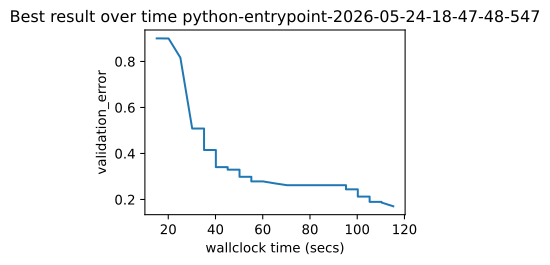
22.5.3 Visualize the Optimization Process
Once more, we visualize the learning curves of every trial (each color in the plot represents a trial). Compare this to asynchronous random search in Section 22.3. As we have seen for successive halving in Section 22.4, most of the trials are stopped at 1 or 2 epochs (\(r_{\mathrm{min}}\) or \(\eta * r_{\mathrm{min}}\)). However, trials do not stop at the same point, because they require different amount of time per epoch. If we ran standard successive halving instead of ASHA, we would need to synchronize our workers, before we can promote configurations to the next rung level.
d2l.set_figsize([6, 2.5])
results = e.results
for trial_id in results.trial_id.unique():
    df = results[results["trial_id"] == trial_id]
    d2l.plt.plot(
        df["st_tuner_time"],
        df["validation_error"],
        marker="o"
    )
d2l.plt.xlabel("wall-clock time")
d2l.plt.ylabel("objective function")
Text(0, 0.5, 'objective function')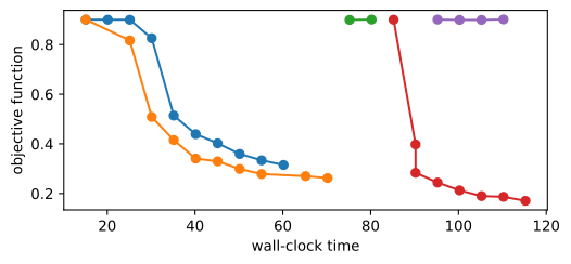
22.5.4 Summary
Compared to random search, successive halving is not quite as trivial to run in an asynchronous distributed setting. To avoid synchronization points, we promote configurations as quickly as possible to the next rung level, even if this means promoting some wrong ones. In practice, this usually does not hurt much, and the gains of asynchronous versus synchronous scheduling are usually much higher than the loss of the suboptimal decision making.