%matplotlib inline
from d2l import torch as d2l
import numpy as np
import pickle
import torch
import torchvision
import warnings
from torch import nn
from torch.nn import functional as F16.5 Adversarial Image Generation
The preceding experiments used two-dimensional distributions, where a scatter plot can reveal whether a generator matches the data. Image generation introduces two additional problems. The generator needs an architecture that maps a latent vector to a \(64 \times 64 \times 3\) array, and visual inspection alone cannot quantify the resulting sample distribution. This section addresses both problems on a dataset of image sprites. We first implement the 2015 DCGAN architecture, then construct a minimal modern backbone on which the classic loss of Section 16.1 and the penalized relativistic loss of Section 16.4 can be compared under identical conditions. We evaluate the two runs with feature-space distances whose closed forms were derived earlier in the chapter.
%matplotlib inline
from d2l import jax as d2l
import jax
from jax import numpy as jnp
from flax import nnx
import numpy as np
import optax
import os
import pickle
import warnings
from PIL import Image
16.5.1 The 2015 Recipe
The original GAN and the Laplacian-pyramid GAN (Denton et al. 2015) had already produced recognizable images, but the classic objective remained difficult to train reliably. The deep convolutional GAN (DCGAN) of Radford et al. (2015) improved reliability through a specific architecture without changing the objective. Its generator upsamples by transposed convolution, its discriminator downsamples by strided convolution, and both networks use batch normalization. The generator uses ReLU activations followed by a tanh output. The discriminator uses leaky ReLU, and Adam uses the reduced momentum parameter \(\beta_1 = 0.5\) (Section 9.6). Batch normalization controls activation scales as both networks change. The tanh output matches the generator’s range to the scaled image data, while reduced momentum shortens the optimizer’s memory in a changing gradient field. The training loss remains the non-saturating log loss of Section 16.1. The controlled comparison later in the section separates architectural stabilization from objective design.
16.5.1.1 The Pokemon Sprites
The dataset contains 40,597 Pokemon sprite images obtained from pokemondb. It covers 721 species, with many variants of each species. Sprites are suitable for a from-scratch experiment because they are small, centered on clean backgrounds, and diverse in silhouette and palette. We resize each image to \(64 \times 64\) with bilinear resampling and scale its pixel values to \([-1, 1]\). Real and generated images then use the same scale, which also matches the range of the 2015 generator’s tanh output. Because the full dataset fits comfortably in memory, we decode it into one tensor and draw subsequent minibatches by indexing.
d2l.DATA_HUB['pokemon'] = (d2l.DATA_URL + 'pokemon.zip',
                           'c065c0e2593b8b161a2d7873e42418bf6a21106c')

data_dir = d2l.download_extract('pokemon')
warnings.filterwarnings('ignore', message='Palette images')
transformer = torchvision.transforms.Compose([
    torchvision.transforms.Resize((64, 64)),
    torchvision.transforms.PILToTensor()])
pokemon = torchvision.datasets.ImageFolder(data_dir, transform=transformer)
loader = torch.utils.data.DataLoader(
    pokemon, batch_size=512, num_workers=d2l.get_dataloader_workers())
images = torch.cat([X for X, _ in loader]).float() / 127.5 - 1
images.shape
torch.Size([40597, 3, 64, 64])
d2l.DATA_HUB['pokemon'] = (d2l.DATA_URL + 'pokemon.zip',
                           'c065c0e2593b8b161a2d7873e42418bf6a21106c')

data_dir = d2l.download_extract('pokemon')
warnings.filterwarnings('ignore', message='Palette images')
files = sorted(os.path.join(root, f)
               for root, _, names in os.walk(data_dir) for f in names
               if f.lower().endswith(('.png', '.jpg', '.jpeg')))
def load_image(path):
    img = Image.open(path).convert('RGB').resize((64, 64), Image.BILINEAR)
    return np.asarray(img, dtype=np.float32) / 127.5 - 1
images = np.stack([load_image(f) for f in files])
images.shape
(40597, 64, 64, 3)A fixed permutation selects one tenth of the images for a held-out set that is never used for training. We use this set both to detect critic overfitting and to evaluate generated samples against unseen real images. Comparing critic scores on the training and held-out sets tests whether the critic has memorized its training images; it does not test whether the generator has copied them. The split is by image rather than species, so variants of one creature may appear in both sets. This dependence limits both uses of the holdout set.
device = d2l.try_gpu()
perm = np.random.RandomState(12345).permutation(len(images))
n_holdout = len(images) // 10
train_imgs = images[perm[n_holdout:]].to(device)
holdout_imgs = images[perm[:n_holdout]].to(device)
print(f'{len(train_imgs)} training and {len(holdout_imgs)} held-out images')
d2l.show_images(train_imgs[:20].cpu().permute(0, 2, 3, 1) / 2 + 0.5,
                num_rows=4, num_cols=5);
36538 training and 4059 held-out images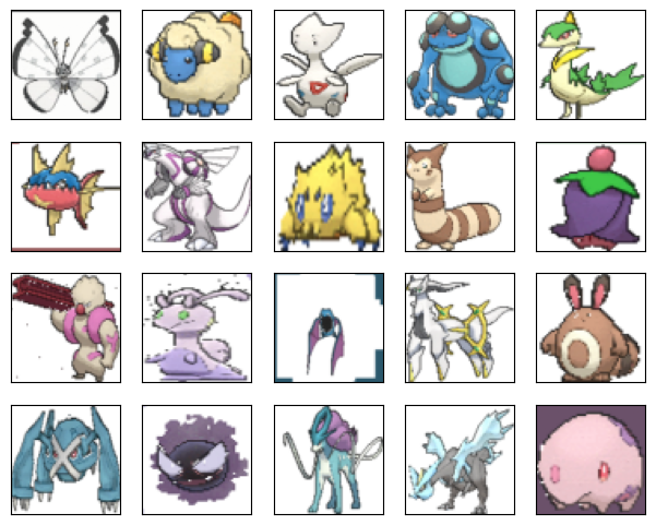
perm = np.random.RandomState(12345).permutation(len(images))
n_holdout = len(images) // 10
train_imgs = jnp.asarray(images[perm[n_holdout:]])
holdout_imgs = jnp.asarray(images[perm[:n_holdout]])
print(f'{len(train_imgs)} training and {len(holdout_imgs)} held-out images')
d2l.show_images(np.asarray(train_imgs[:20]) / 2 + 0.5,
                num_rows=4, num_cols=5);
36538 training and 4059 held-out images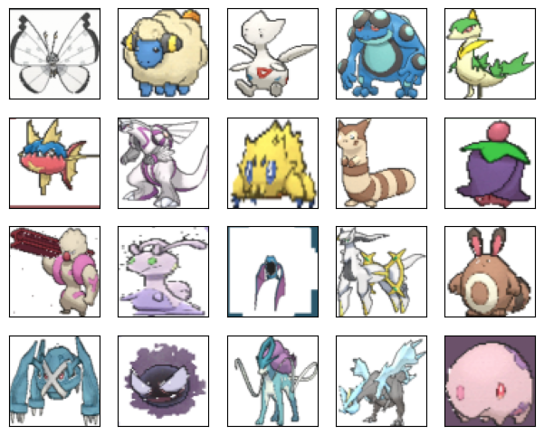
16.5.1.2 Generator
The generator must turn a latent vector, treated as a \(1 \times 1\) image with 100 channels, into a \(64 \times 64\) image with 3 channels: a factor of 64 in each spatial dimension. The DCGAN building block grows the resolution with a transposed convolution (Section 20.10), the upsampling layer that Section 20.11 used to enlarge feature maps, followed by batch normalization and a ReLU.
class G_block(nn.Module):
    def __init__(self, out_channels, in_channels=3, kernel_size=4, strides=2,
                 padding=1):
        super().__init__()
        self.conv2d_trans = nn.ConvTranspose2d(
            in_channels, out_channels, kernel_size, strides, padding,
            bias=False)
        self.batch_norm = nn.BatchNorm2d(out_channels)
        self.activation = nn.ReLU()

    def forward(self, X):
        return self.activation(self.batch_norm(self.conv2d_trans(X)))
def bn_scale_init(key, shape, dtype=jnp.float32):
"""DCGAN initialization for batch-norm scales: N(1, 0.02^2)."""
return 1 + 0.02 * jax.random.normal(key, shape, dtype)
class G_block(nnx.Module):
def __init__(self, out_channels, in_channels=3, kernel_size=4,
strides=2, padding='SAME', rngs=None):
rngs = nnx.Rngs(d2l.get_key()) if rngs is None else rngs
self.conv2d_trans = nnx.ConvTranspose(
in_channels, out_channels,
kernel_size=(kernel_size, kernel_size),
strides=(strides, strides), padding=padding, use_bias=False,
kernel_init=nnx.initializers.normal(0.02), rngs=rngs)
self.batch_norm = nnx.BatchNorm(out_channels,
scale_init=bn_scale_init, rngs=rngs)
def __call__(self, X):
return nnx.relu(self.batch_norm(self.conv2d_trans(X)))The transposed-convolution dimensions determine the spatial layout. With kernel size \(k\), stride \(s\), and padding \(p\), an \(n \times n\) input produces an output of side \(s(n - 1) + k - 2p\). The default block uses \(k = 4\), \(s = 2\), \(p = 1\), so the output side is \(2n\): each block exactly doubles the resolution. With \(s = 1\) and \(p = 0\), the same kernel maps a \(1 \times 1\) input to a \(4 \times 4\) feature map, which provides the generator’s initial spatial representation.
print(G_block(20)(torch.zeros((2, 3, 16, 16))).shape)
print(G_block(20, strides=1, padding=0)(torch.zeros((2, 3, 1, 1))).shape)
torch.Size([2, 20, 32, 32])
torch.Size([2, 20, 4, 4])print(G_block(20, rngs=nnx.Rngs(0))(jnp.zeros((2, 16, 16, 3))).shape)
print(G_block(20, strides=1, padding='VALID',
rngs=nnx.Rngs(0))(jnp.zeros((2, 1, 1, 3))).shape)(2, 32, 32, 20)
(2, 4, 4, 20)The full generator chains these blocks through \(4 \to 8 \to 16 \to 32 \to 64\). The first block maps the latent input to \(4 \times 4\) at \(64 \cdot 8\) channels, and three more blocks double the resolution to \(32 \times 32\) while halving the channels each time. A final transposed convolution performs the last doubling to \(64 \times 64\) while projecting to 3 channels, and a tanh squashes the output into \([-1, 1]\).
n_G = 64
net_G = nn.Sequential(
    G_block(in_channels=100, out_channels=n_G * 8,
            strides=1, padding=0),                   # Output: (64 * 8, 4, 4)
    G_block(in_channels=n_G * 8, out_channels=n_G * 4),  # (64 * 4, 8, 8)
    G_block(in_channels=n_G * 4, out_channels=n_G * 2),  # (64 * 2, 16, 16)
    G_block(in_channels=n_G * 2, out_channels=n_G),      # (64, 32, 32)
    nn.ConvTranspose2d(in_channels=n_G, out_channels=3, kernel_size=4,
                       stride=2, padding=1, bias=False),
    nn.Tanh())                                           # Output: (3, 64, 64)
net_G(torch.zeros((1, 100, 1, 1))).shape
torch.Size([1, 3, 64, 64])n_G = 64
class DCGANGenerator(nnx.Module):
def __init__(self, latent_dim=100, n_G=64, rngs=None):
rngs = nnx.Rngs(d2l.get_key()) if rngs is None else rngs
self.blocks = nnx.List([
G_block(n_G * 8, latent_dim, strides=1, padding='VALID',
rngs=rngs), # Output: (4, 4, 64 * 8)
G_block(n_G * 4, n_G * 8, rngs=rngs), # (8, 8, 64 * 4)
G_block(n_G * 2, n_G * 4, rngs=rngs), # (16, 16, 64 * 2)
G_block(n_G, n_G * 2, rngs=rngs)]) # (32, 32, 64)
self.output = nnx.ConvTranspose(
n_G, 3, kernel_size=(4, 4), strides=(2, 2), padding='SAME',
use_bias=False, kernel_init=nnx.initializers.normal(0.02),
rngs=rngs)
def __call__(self, X):
for block in self.blocks:
X = block(X)
return nnx.tanh(self.output(X)) # Output: (64, 64, 3)
net_G = DCGANGenerator(n_G=n_G, rngs=nnx.Rngs(0))
net_G(jnp.zeros((1, 1, 1, 100))).shape(1, 64, 64, 3)16.5.1.3 Discriminator
The discriminator runs the same pipeline in reverse: ordinary strided convolutions halve the resolution block by block until a final \(4 \times 4\) convolution produces a single realness logit. Its activation is the leaky ReLU,
\[\textrm{leaky ReLU}(x) = \begin{cases}x & \textrm{if}\ x > 0,\\ \alpha x & \textrm{otherwise},\end{cases} \tag{16.5.1}\]
with slope \(\alpha \in (0, 1)\) on the negative side. An ordinary ReLU passes zero gradient whenever its input is negative. A discriminator unit that remains in this regime supplies no gradient to the generator. The nonzero negative slope preserves that gradient path, which is especially important because the generator learns only through derivatives of the discriminator.
class D_block(nn.Module):
    def __init__(self, out_channels, in_channels=3, kernel_size=4, strides=2,
                 padding=1, alpha=0.2):
        super().__init__()
        self.conv2d = nn.Conv2d(in_channels, out_channels, kernel_size,
                                strides, padding, bias=False)
        self.batch_norm = nn.BatchNorm2d(out_channels)
        self.activation = nn.LeakyReLU(alpha)

    def forward(self, X):
        return self.activation(self.batch_norm(self.conv2d(X)))
class D_block(nnx.Module):
def __init__(self, out_channels, in_channels=3, kernel_size=4,
strides=2, padding='SAME', alpha=0.2, rngs=None):
rngs = nnx.Rngs(d2l.get_key()) if rngs is None else rngs
self.alpha = alpha
self.conv2d = nnx.Conv(
in_channels, out_channels,
kernel_size=(kernel_size, kernel_size),
strides=(strides, strides), padding=padding, use_bias=False,
kernel_init=nnx.initializers.normal(0.02), rngs=rngs)
self.batch_norm = nnx.BatchNorm(out_channels,
scale_init=bn_scale_init, rngs=rngs)
def __call__(self, X):
return nnx.leaky_relu(self.batch_norm(self.conv2d(X)),
negative_slope=self.alpha)With the same \(k = 4\), \(s = 2\), \(p = 1\) configuration, the ordinary convolution’s output side is \(\lfloor (n - k + 2p + s)/s \rfloor = n/2\) for even \(n\). Four blocks therefore reduce \(64 \times 64\) to \(4 \times 4\) while the channel count doubles per block, and a final unpadded \(4 \times 4\) convolution maps the result to a single scalar.
n_D = 64
net_D = nn.Sequential(
    D_block(n_D),                                    # Output: (64, 32, 32)
    D_block(in_channels=n_D, out_channels=n_D * 2),  # (64 * 2, 16, 16)
    D_block(in_channels=n_D * 2, out_channels=n_D * 4),  # (64 * 4, 8, 8)
    D_block(in_channels=n_D * 4, out_channels=n_D * 8),  # (64 * 8, 4, 4)
    nn.Conv2d(in_channels=n_D * 8, out_channels=1,
              kernel_size=4, bias=False))            # Output: (1, 1, 1)
net_D(torch.zeros((1, 3, 64, 64))).shape
torch.Size([1, 1, 1, 1])n_D = 64
class DCGANDiscriminator(nnx.Module):
def __init__(self, n_D=64, rngs=None):
rngs = nnx.Rngs(d2l.get_key()) if rngs is None else rngs
self.blocks = nnx.List([
D_block(n_D, 3, rngs=rngs), # Output: (32, 32, 64)
D_block(n_D * 2, n_D, rngs=rngs), # (16, 16, 64 * 2)
D_block(n_D * 4, n_D * 2, rngs=rngs), # (8, 8, 64 * 4)
D_block(n_D * 8, n_D * 4, rngs=rngs)]) # (4, 4, 64 * 8)
self.output = nnx.Conv(
n_D * 8, 1, kernel_size=(4, 4), padding='VALID', use_bias=False,
kernel_init=nnx.initializers.normal(0.02), rngs=rngs)
def __call__(self, X):
for block in self.blocks:
X = block(X)
return self.output(X) # Output: (1, 1, 1)
net_D = DCGANDiscriminator(n_D=n_D, rngs=nnx.Rngs(1))
net_D(jnp.zeros((1, 64, 64, 3))).shape(1, 1, 1, 1)16.5.1.4 Training with the Classic Loss
The library functions from Section 16.1 also apply to images. The function d2l.update_D ascends the log-loss objective Equation 16.1.1, and d2l.update_G descends the non-saturating generator loss from Equation 16.1.5. The loop below alternates these updates over shuffled minibatches, with the shared learning rate and \(\beta_1 = 0.5\) prescribed by DCGAN. Initialization also follows the DCGAN convention. Convolution and transposed-convolution kernels are drawn from \(\mathcal{N}(0, 0.02^2)\), batch-normalization scales from \(\mathcal{N}(1, 0.02^2)\), and all offsets start at zero. PyTorch applies this convention through dcgan_init; JAX uses the initializers declared in the preceding blocks.
def dcgan_init(module):
    """DCGAN initialization by role: conv kernels N(0, 0.02^2),
    batch-norm scales N(1, 0.02^2), offsets zero."""
    if isinstance(module, (nn.Conv2d, nn.ConvTranspose2d)):
        nn.init.normal_(module.weight, 0, 0.02)
    elif isinstance(module, nn.BatchNorm2d):
        nn.init.normal_(module.weight, 1, 0.02)
        nn.init.zeros_(module.bias)

def train_dcgan(net_D, net_G, num_epochs=20, batch_size=256, lr=0.0002,
                latent_dim=100):
    loss = nn.BCEWithLogitsLoss(reduction='mean')
    for net in (net_D, net_G):
        net.apply(dcgan_init)
    net_D, net_G = net_D.to(device), net_G.to(device)
    trainer_D = torch.optim.Adam(net_D.parameters(), lr=lr,
                                 betas=(0.5, 0.999))
    trainer_G = torch.optim.Adam(net_G.parameters(), lr=lr,
                                 betas=(0.5, 0.999))
    history = []
    for epoch in range(num_epochs):
        metric = d2l.Accumulator(3)
        order = torch.randperm(len(train_imgs), device=device)
        for i in range(0, len(order) - batch_size + 1, batch_size):
            X = train_imgs[order[i:i + batch_size]]
            Z = torch.randn(batch_size, latent_dim, 1, 1, device=device)
            metric.add(
                d2l.update_D(X, Z, net_D, net_G, loss, trainer_D).detach(),
                d2l.update_G(Z, net_D, net_G, loss, trainer_G).detach(), 1)
        history.append((metric[0] / metric[2], metric[1] / metric[2]))
    return history
def train_dcgan(net_D, net_G, num_epochs=20, batch_size=256, lr=0.0002,
latent_dim=100):
optimizer_D = nnx.Optimizer(net_D, optax.adam(lr, b1=0.5, b2=0.999),
wrt=nnx.Param)
optimizer_G = nnx.Optimizer(net_G, optax.adam(lr, b1=0.5, b2=0.999),
wrt=nnx.Param)
key = jax.random.PRNGKey(0)
history = []
for epoch in range(num_epochs):
key, kp = jax.random.split(key)
order = jax.random.permutation(kp, len(train_imgs))
loss_D_sum, loss_G_sum, steps = 0.0, 0.0, 0
for i in range(0, len(order) - batch_size + 1, batch_size):
X = train_imgs[order[i:i + batch_size]]
key, kz = jax.random.split(key)
Z = jax.random.normal(kz, (batch_size, 1, 1, latent_dim))
loss_D_sum += d2l.update_D(X, Z, net_D, net_G, optimizer_D)
loss_G_sum += d2l.update_G(Z, net_D, net_G, optimizer_G)
steps += 1
history.append((float(loss_D_sum) / (steps * batch_size),
float(loss_G_sum) / (steps * batch_size)))
return historyTwenty epochs take a few minutes on one GPU.
history = train_dcgan(net_D, net_G)
print(f'final loss_D {history[-1][0]:.3f}, loss_G {history[-1][1]:.3f}')
final loss_D 0.181, loss_G 3.066history = train_dcgan(net_D, net_G)
print(f'final loss_D {history[-1][0]:.3f}, loss_G {history[-1][1]:.3f}')final loss_D 0.153, loss_G 3.209with torch.no_grad():
fake = net_G(torch.randn(20, 100, 1, 1, device=device))
d2l.show_images(fake.cpu().permute(0, 2, 3, 1) / 2 + 0.5,
num_rows=4, num_cols=5);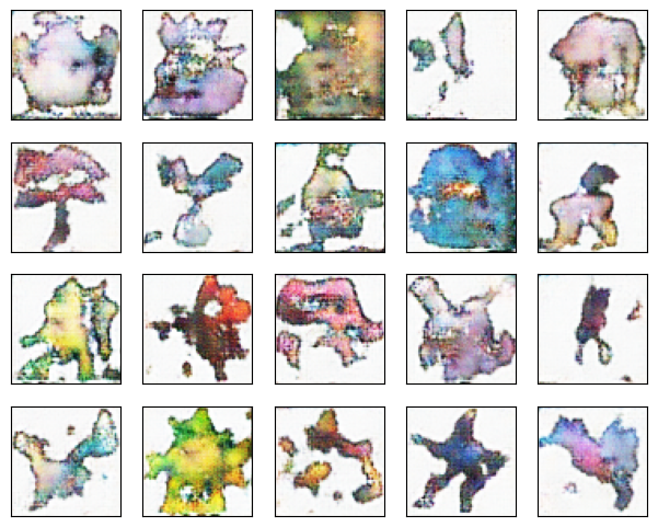
fake = net_G(jax.random.normal(jax.random.PRNGKey(2), (20, 1, 1, 100)))
d2l.show_images(np.asarray(fake) / 2 + 0.5, num_rows=4, num_cols=5);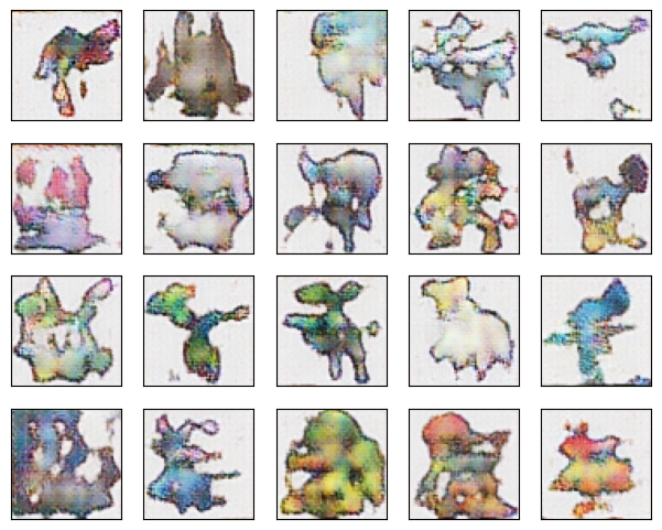
The samples reproduce several visible properties of the dataset: centered shapes, plausible palettes, rough silhouettes, and clean backgrounds. DCGAN made the classic objective practical for image generation, but its architecture does not alter that objective. The mode-dropping minima of Section 16.3 and the divergent dynamics of Section 16.4 therefore remain possible. DCGAN remains sensitive to hyperparameters and may collapse during longer runs. To compare objectives directly, we next use a backbone without normalization or other DCGAN-specific stabilizers.
16.5.2 A Modern Minimal Backbone
The R3GAN recipe of Section 16.4 combines the pairing loss and two zero-centered penalties with a simpler architecture. At the scale of the sprite experiment, we use bilinear interpolation followed by an ordinary \(3 \times 3\) convolution for both upsampling and downsampling. This replaces strided and transposed convolutions, whose uneven kernel overlap can produce checkerboard artifacts (Odena et al. 2016). Both networks use leaky ReLU throughout, and the generator has no tanh output. Neither network uses normalization. Batch normalization would make each critic score depend on the entire minibatch, coupling the per-sample input gradients in Equation 16.4.4 and confounding the penalty with a second stabilizer. Removing normalization also eliminates running statistics and the distinction between training and evaluation modes, so the update rules of Section 16.1 apply without special cases.
The modern generator begins from a learned \(4 \times 4 \times 128\) constant rather than from the latent vector, so it needs a separate path for the latent code. R3GAN’s Config E uses a basis layer: a linear function of \(z\) modulates learned \(4 \times 4\) feature maps. We use a simpler mechanism. A linear layer projects \(z\) to a \(4 \times 4 \times 100\) map, which is concatenated with the learned constant along the channel axis. A \(3 \times 3\) convolution mixes the two inputs before upsampling begins. Concatenation costs less than modulation and leaves the constant unchanged. The constant represents features shared across samples, whereas the projected latent code supplies the per-sample variation.
class Generator(nn.Module):
    """Learned 4x4 constant + projected latent, bilinearly upsampled."""
    def __init__(self, latent_dim=100, const_ch=128, base_ch=512):
        super().__init__()
        self.latent_dim = latent_dim
        self.const = nn.Parameter(0.02 * torch.randn(1, const_ch, 4, 4))
        self.z_proj = nn.Linear(latent_dim, 16 * latent_dim)
        self.mix = nn.Conv2d(const_ch + latent_dim, base_ch, 3, padding=1)
        chans = [base_ch // 2 ** i for i in range(5)]    # 512, 256, ..., 32
        self.stages = nn.ModuleList(
            [nn.Conv2d(c_in, c_out, 3, padding=1)
             for c_in, c_out in zip(chans[:-1], chans[1:])])
        self.to_rgb = nn.Conv2d(chans[-1], 3, 3, padding=1)
        self.act = nn.LeakyReLU(0.2)

    def forward(self, z):
        zc = self.z_proj(z).reshape(-1, self.latent_dim, 4, 4)
        const = self.const.expand(z.shape[0], -1, -1, -1)
        x = self.act(self.mix(torch.cat([const, zc], dim=1)))
        for conv in self.stages:                     # 4 -> 8 -> ... -> 64
            x = F.interpolate(x, scale_factor=2, mode='bilinear')
            x = self.act(conv(x))
        return self.to_rgb(x)                        # no tanh: raw output
class Generator(nnx.Module):
"""Learned 4x4 constant + projected latent, bilinearly upsampled."""
def __init__(self, latent_dim=100, const_ch=128, base_ch=512,
rngs=None):
rngs = nnx.Rngs(d2l.get_key()) if rngs is None else rngs
self.latent_dim = latent_dim
init = nnx.initializers.normal(0.02)
self.const = nnx.Param(init(rngs.params(), (1, 4, 4, const_ch)))
self.z_proj = nnx.Linear(latent_dim, 16 * latent_dim,
kernel_init=init, rngs=rngs)
self.mix = nnx.Conv(const_ch + latent_dim, base_ch, (3, 3),
padding='SAME', kernel_init=init, rngs=rngs)
chans = [base_ch // 2 ** i for i in range(5)] # 512, 256, ..., 32
self.stages = nnx.List(
[nnx.Conv(c_in, c_out, (3, 3), padding='SAME',
kernel_init=init, rngs=rngs)
for c_in, c_out in zip(chans[:-1], chans[1:])])
self.to_rgb = nnx.Conv(chans[-1], 3, (3, 3), padding='SAME',
kernel_init=init, rngs=rngs)
def __call__(self, z):
zc = self.z_proj(z).reshape(-1, 4, 4, self.latent_dim)
const = jnp.broadcast_to(self.const[...],
(z.shape[0],) + self.const.shape[1:])
x = nnx.leaky_relu(self.mix(jnp.concatenate([const, zc], axis=-1)),
0.2)
for conv in self.stages: # 4 -> 8 -> ... -> 64
b, h, w, c = x.shape
x = jax.image.resize(x, (b, 2 * h, 2 * w, c), method='bilinear')
x = nnx.leaky_relu(conv(x), 0.2)
return self.to_rgb(x) # no tanh: raw outputThe critic reverses the generator’s resolution schedule. Four stages of convolution, leaky ReLU, and bilinear downsampling reduce a \(64 \times 64\) image to a \(4 \times 4\) feature map while increasing the channel count. A mixing convolution widens the final map, and a linear head produces one scalar. This mirrored design gives the two networks comparable resolution schedules and capacities.
class Discriminator(nn.Module):
    """Mirror of the generator: conv + leaky ReLU + bilinear downsampling."""
    def __init__(self, base_ch=32):
        super().__init__()
        chans = [3] + [base_ch * 2 ** i for i in range(4)]  # 3, 32, ..., 256
        self.stages = nn.ModuleList(
            [nn.Conv2d(c_in, c_out, 3, padding=1)
             for c_in, c_out in zip(chans[:-1], chans[1:])])
        self.mix = nn.Conv2d(chans[-1], 2 * chans[-1], 3, padding=1)
        self.head = nn.Linear(2 * chans[-1] * 4 * 4, 1)
        self.act = nn.LeakyReLU(0.2)

    def forward(self, x):
        for conv in self.stages:                     # 64 -> 32 -> ... -> 4
            x = F.interpolate(self.act(conv(x)), scale_factor=0.5,
                              mode='bilinear', antialias=True)
        x = self.act(self.mix(x))
        return self.head(x.reshape(x.shape[0], -1))

for net in (Generator(), Discriminator()):
    print(f'{type(net).__name__}: '
          f'{sum(p.numel() for p in net.parameters())} parameters')
Generator: 2782851 parameters
Discriminator: 1576769 parametersclass Discriminator(nnx.Module):
"""Mirror of the generator: conv + leaky ReLU + bilinear downsampling."""
def __init__(self, base_ch=32, rngs=None):
rngs = nnx.Rngs(d2l.get_key()) if rngs is None else rngs
init = nnx.initializers.normal(0.02)
chans = [3] + [base_ch * 2 ** i for i in range(4)] # 3, 32, ..., 256
self.stages = nnx.List(
[nnx.Conv(c_in, c_out, (3, 3), padding='SAME',
kernel_init=init, rngs=rngs)
for c_in, c_out in zip(chans[:-1], chans[1:])])
self.mix = nnx.Conv(chans[-1], 2 * chans[-1], (3, 3),
padding='SAME', kernel_init=init, rngs=rngs)
self.head = nnx.Linear(2 * chans[-1] * 4 * 4, 1,
kernel_init=init, rngs=rngs)
def __call__(self, x):
for conv in self.stages: # 64 -> 32 -> ... -> 4
x = nnx.leaky_relu(conv(x), 0.2)
b, h, w, c = x.shape
x = jax.image.resize(x, (b, h // 2, w // 2, c),
method='bilinear')
x = nnx.leaky_relu(self.mix(x), 0.2)
return self.head(x.reshape(x.shape[0], -1))
for net in (Generator(rngs=nnx.Rngs(0)), Discriminator(rngs=nnx.Rngs(0))):
n = sum(v.size for v in jax.tree.leaves(nnx.state(net, nnx.Param)))
print(f'{type(net).__name__}: {n} parameters')Generator: 2782851 parameters
Discriminator: 1576769 parametersThe generator has about 2.8 million parameters and the critic about 1.6 million. This model is a reduced instance of the R3GAN design rather than the published Config E. We omit its grouped convolutions, inverted bottlenecks, and additional residual depth, which provide capacity at the larger scale considered in that work.
Two additional training choices complete the recipe. First, random horizontal flips augment the real images. A critic with enough capacity can memorize a dataset of this size, and augmentation reduces that risk; Karras, Aittala, et al. (2020) develops a feedback-controlled version for larger models. Second, evaluation uses an exponential moving average of the generator parameters rather than the raw iterates. This is the weight EMA introduced for classifiers in Equation 7.6.5. The two-player dynamics analyzed in Section 16.4 rotate while contracting, so averaging successive iterates also reduces their displacement from the equilibrium. We use a half-life of 500 steps.
class EMA:
    """Exponential moving average of model weights, given as a half-life."""
    def __init__(self, model, half_life):
        self.shadow = {k: v.detach().clone()
                       for k, v in model.state_dict().items()}
        self.decay = 0.5 ** (1 / half_life)

    def update(self, model):
        with torch.no_grad():
            for k, v in model.state_dict().items():
                self.shadow[k].lerp_(v, 1 - self.decay)

    def copy_to(self, model):
        model.load_state_dict(self.shadow)

def sample_real(images, n):
    """Draw a training batch with random horizontal flips."""
    idx = torch.randint(0, len(images), (n,), device=images.device)
    batch = images[idx]
    flip = torch.rand(n, device=images.device) < 0.5
    return torch.where(flip.view(-1, 1, 1, 1), batch.flip(-1), batch)
class EMA:
"""Exponential moving average of model weights, given as a half-life."""
def __init__(self, model, half_life):
self.shadow = jax.tree.map(jnp.copy, nnx.state(model, nnx.Param))
self.decay = 0.5 ** (1 / half_life)
def update(self, model):
self.shadow = jax.tree.map(
lambda s, p: self.decay * s + (1 - self.decay) * p,
self.shadow, nnx.state(model, nnx.Param))
def copy_to(self, model):
nnx.update(model, self.shadow)
def sample_real(key, images, n):
"""Draw a training batch with random horizontal flips."""
k1, k2 = jax.random.split(key)
idx = jax.random.randint(k1, (n,), 0, len(images))
batch = images[idx]
flip = jax.random.bernoulli(k2, 0.5, (n,))
return jnp.where(flip[:, None, None, None], batch[:, :, ::-1, :], batch)16.5.3 Loss A/B on One Backbone
The controlled comparison uses two training arms with the same backbone and initialization. Every convolutional and linear weight is drawn from \(\mathcal{N}(0, 0.02^2)\), following the 2015 convention, and every bias starts at zero. Both frameworks apply the same role-aware convention used for DCGAN above; because this backbone has no normalization parameters, the roles reduce to weights and biases. Within each framework, the two arms therefore begin with identical parameters. Across frameworks, the backbones have the same layers, initialization convention, and antialiased bilinear downsampling, but they are not bitwise identical because each library uses its own random stream.
The arms share Adam with \(\beta_1 = 0\) and \(\beta_2 = 0.99\) at learning rate \(2 \cdot 10^{-4}\), batch size 64, augmentation, EMA, and a budget of 15,000 steps, or about 26 epochs. They differ only in the loss. The first arm uses the classic non-saturating objective through d2l.update_D and d2l.update_G. The second uses the loss from Section 16.4: the relativistic pairing objective with its non-saturating generator, d2l.rpgan_loss_D and d2l.rpgan_loss_G, plus both zero-centered penalties from d2l.r1_r2_penalty.
We set the penalty weight to \(\gamma = 10\) after sweeping powers of ten on this dataset. Weights from 1 to 100 train stably, whereas \(\gamma = 0.1\) under-damps the game and leads to collapse. This stable range is specific to the experiment. Across the R3GAN benchmarks, the tuned value ranges from 0.05 on CIFAR-10 to 150 on FFHQ-256 (Huang et al. 2024). A value chosen on one dataset therefore provides only an order-of-magnitude starting point for another.
def train_backbone(loss_type, gamma=10, num_steps=15000, batch_size=64,
                   lr=0.0002, latent_dim=100, half_life=500, log_every=250):
    torch.manual_seed(0)
    net_G, net_D = Generator().to(device), Discriminator().to(device)
    def init_weights(module):
        if isinstance(module, (nn.Conv2d, nn.Linear)):
            nn.init.normal_(module.weight, 0, 0.02)
            nn.init.zeros_(module.bias)
    for net in (net_G, net_D):
        net.apply(init_weights)
    trainer_G = torch.optim.Adam(net_G.parameters(), lr=lr,
                                 betas=(0.0, 0.99))
    trainer_D = torch.optim.Adam(net_D.parameters(), lr=lr,
                                 betas=(0.0, 0.99))
    loss = nn.BCEWithLogitsLoss(reduction='mean')
    ema, history = EMA(net_G, half_life), []
    for step in range(1, num_steps + 1):
        X = sample_real(train_imgs, batch_size)
        Z = torch.randn(batch_size, latent_dim, device=device)
        Z2 = torch.randn(batch_size, latent_dim, device=device)
        if loss_type == 'classic':
            loss_D = d2l.update_D(X, Z, net_D, net_G, loss, trainer_D)
            loss_G = d2l.update_G(Z2, net_D, net_G, loss, trainer_G)
        else:
            fake = net_G(Z).detach()
            r1, r2 = d2l.r1_r2_penalty(net_D, X, fake)
            loss_D = (d2l.rpgan_loss_D(net_D, X, fake)
                      + gamma / 2 * (r1 + r2).mean())
            trainer_D.zero_grad(), loss_D.backward(), trainer_D.step()
            loss_G = d2l.rpgan_loss_G(net_D, sample_real(train_imgs,
                                                         batch_size),
                                      net_G(Z2))
            trainer_G.zero_grad(), loss_G.backward(), trainer_G.step()
        ema.update(net_G)
        if step % log_every == 0:
            with torch.no_grad():
                d_real = net_D(sample_real(train_imgs, 256)).mean()
            history.append((step, float(loss_D.detach()),
                            float(loss_G.detach()), float(d_real)))
    ema_G = Generator().to(device)
    ema.copy_to(ema_G)
    return ema_G, net_D, torch.tensor(history)
@nnx.jit
def rpgan_step(net_G, net_D, opt_G, opt_D, X, Z, X2, Z2, gamma):
def loss_D_fn(net_D):
fake = jax.lax.stop_gradient(net_G(Z))
r1, r2 = d2l.r1_r2_penalty(net_D, X, fake)
return (d2l.rpgan_loss_D(net_D, X, fake)
+ gamma / 2 * (r1 + r2).mean())
loss_D, grads = nnx.value_and_grad(loss_D_fn)(net_D)
opt_D.update(net_D, grads)
def loss_G_fn(net_G):
return d2l.rpgan_loss_G(net_D, X2, net_G(Z2))
loss_G, grads = nnx.value_and_grad(loss_G_fn)(net_G)
opt_G.update(net_G, grads)
return loss_D, loss_G
def train_backbone(loss_type, gamma=10.0, num_steps=15000, batch_size=64,
lr=0.0002, latent_dim=100, half_life=500, log_every=250):
rngs = nnx.Rngs(0)
net_G, net_D = Generator(rngs=rngs), Discriminator(rngs=rngs)
opt_G = nnx.Optimizer(net_G, optax.adam(lr, b1=0.0, b2=0.99),
wrt=nnx.Param)
opt_D = nnx.Optimizer(net_D, optax.adam(lr, b1=0.0, b2=0.99),
wrt=nnx.Param)
ema, history = EMA(net_G, half_life), []
key = jax.random.PRNGKey(1)
for step in range(1, num_steps + 1):
key, kx, kz, kx2, kz2, kd = jax.random.split(key, 6)
X = sample_real(kx, train_imgs, batch_size)
Z = jax.random.normal(kz, (batch_size, latent_dim))
Z2 = jax.random.normal(kz2, (batch_size, latent_dim))
if loss_type == 'classic':
loss_D = d2l.update_D(X, Z, net_D, net_G, opt_D) / batch_size
loss_G = d2l.update_G(Z2, net_D, net_G, opt_G) / batch_size
else:
X2 = sample_real(kx2, train_imgs, batch_size)
loss_D, loss_G = rpgan_step(net_G, net_D, opt_G, opt_D,
X, Z, X2, Z2, gamma)
ema.update(net_G)
if step % log_every == 0:
d_real = net_D(sample_real(kd, train_imgs, 256)).mean()
history.append((step, float(loss_D), float(loss_G),
float(d_real)))
ema_G = Generator(rngs=nnx.Rngs(0))
ema.copy_to(ema_G)
return ema_G, net_D, np.array(history)These two runs are the longest computation in the chapter. The penalized arm costs more because the penalty differentiates the critic’s input gradient a second time. On one RTX 4090, the pair takes twenty to thirty minutes in PyTorch and about half that time in JAX; peak memory remains modest at batch size 64. After each run, we compare the critic’s mean score on training and held-out images. A positive training–holdout gap is evidence that the critic distinguishes its training set from unseen images, whereas a gap near zero shows no such difference in the mean score. This statistic does not determine whether the generator memorizes training images. Section 16.5.5.1 tests generator memorization directly by comparing generated samples with their nearest training images.
runs = {}
for name, loss_type in [('classic', 'classic'), ('RpGAN + R1 + R2', 'rp')]:
    ema_G, net_D_run, hist = train_backbone(loss_type)
    with torch.no_grad():
        gap = (net_D_run(train_imgs[:1024]).mean()
               - net_D_run(holdout_imgs[:1024]).mean())
    runs[name] = (ema_G, hist)
    print(f'{name}: final loss_D {hist[-1, 1]:.3f}, '
          f'loss_G {hist[-1, 2]:.3f}, '
          f'critic train-holdout gap {float(gap):+.3f}')
classic: final loss_D 3.119, loss_G 5.710, critic train-holdout gap +0.091
RpGAN + R1 + R2: final loss_D 0.578, loss_G 1.068, critic train-holdout gap -0.019runs = {}
for name, loss_type in [('classic', 'classic'), ('RpGAN + R1 + R2', 'rp')]:
ema_G, net_D_run, hist = train_backbone(loss_type)
gap = (net_D_run(train_imgs[:1024]).mean()
- net_D_run(holdout_imgs[:1024]).mean())
runs[name] = (ema_G, hist)
print(f'{name}: final loss_D {hist[-1, 1]:.3f}, '
f'loss_G {hist[-1, 2]:.3f}, '
f'critic train-holdout gap {float(gap):+.3f}')classic: final loss_D 0.054, loss_G 6.222, critic train-holdout gap +1.053
RpGAN + R1 + R2: final loss_D 0.568, loss_G 1.115, critic train-holdout gap -0.011The grids below provide the first comparison. Both panels show 64 samples from the EMA generator, drawn from the same latent codes in both arms.
def image_grid(imgs, rows=8, cols=8):
    imgs = (imgs.clamp(-1, 1) + 1) / 2
    imgs = imgs.reshape(rows, cols, 3, 64, 64).permute(0, 3, 1, 4, 2)
    return imgs.reshape(rows * 64, cols * 64, 3).cpu().numpy()

torch.manual_seed(42)
z_show = torch.randn(64, 100, device=device)
fig, axes = d2l.plt.subplots(1, 2, figsize=(9, 4.8))
for ax, (name, (ema_G, hist)) in zip(axes, runs.items()):
    with torch.no_grad():
        ax.imshow(image_grid(ema_G(z_show)))
    ax.set_title(name)
    ax.axis('off')
fig.tight_layout()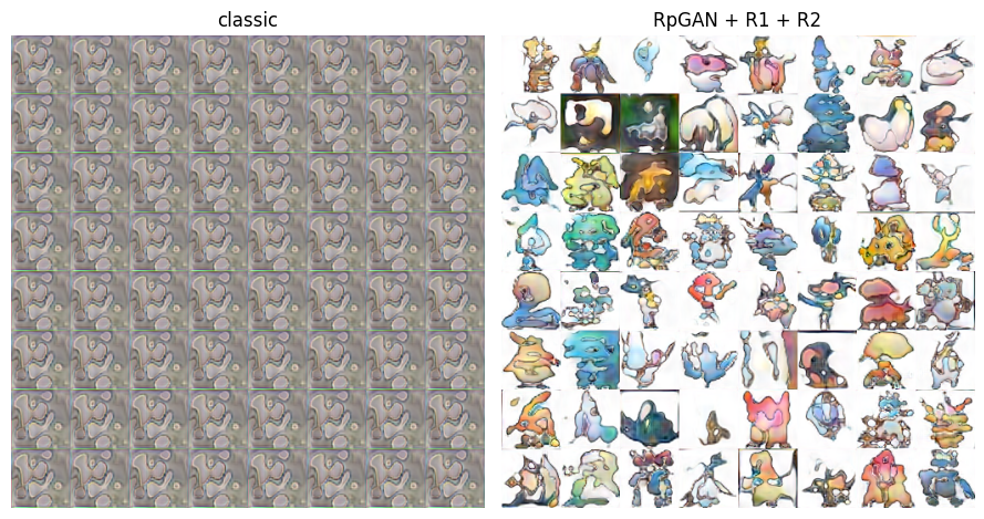
def image_grid(imgs, rows=8, cols=8):
    imgs = (jnp.clip(imgs, -1, 1) + 1) / 2
    imgs = imgs.reshape(rows, cols, 64, 64, 3).transpose(0, 2, 1, 3, 4)
    return np.asarray(imgs.reshape(rows * 64, cols * 64, 3))

z_show = jax.random.normal(jax.random.PRNGKey(42), (64, 100))
fig, axes = d2l.plt.subplots(1, 2, figsize=(9, 4.8))
for ax, (name, (ema_G, hist)) in zip(axes, runs.items()):
    ax.imshow(image_grid(ema_G(z_show)))
    ax.set_title(name)
    ax.axis('off')
fig.tight_layout()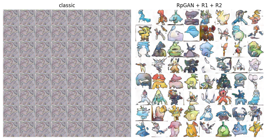
The classic arm collapses: all 64 latent codes produce visually indistinguishable images. This is the most extreme form of mode collapse and corresponds to one of the mode-dropping minima identified in Section 16.3. The result depends on initialization. With either framework’s default initialization, the classic arm remains diverse over this training budget; Exercise 5 performs that control. The \(\mathcal{N}(0, 0.02^2)\) initialization inherited from DCGAN instead leads optimization to a mode-dropping minimum. Because the classic objective does not exclude such minima, different starting points can produce different endpoints.
From the same initialization and with the same training budget, the penalized relativistic arm produces diverse, creature-shaped sprites. The silhouettes and palettes vary, no duplicate is visible, and the grid contains no checkerboard texture. The best-response analysis in Section 16.3 shows that the pairing objective removes collapsed configurations from the set of minima (Huang et al. 2024). This comparison changes the complete loss recipe, adding both the pairing objective and the two penalties, so it does not isolate their individual effects. The three-configuration experiment in Section 16.4 and the StackedMNIST ablation cited there separate these components.
The penalized arm has a train–holdout gap near zero, so its critic assigns similar mean scores to the two splits. The classic arm has a positive gap, but its critic also operates on a much larger score scale; the gap magnitudes are therefore not directly comparable. Neither statistic tests whether the generator memorizes training images. The nearest-neighbor comparison in Section 16.5.5.1 addresses that question. A second seed reproduces both training outcomes.
The grids record only the endpoint of each run. The loss traces below show the dynamics that produced it.
fig, axes = d2l.plt.subplots(1, 3, figsize=(10.5, 3.2))
for ax, (name, (ema_G, hist)) in zip(axes[:2], runs.items()):
    ax.plot(hist[:, 0], hist[:, 1], label='discriminator')
    ax.plot(hist[:, 0], hist[:, 2], label='generator')
    ax.set_title(name), ax.set_xlabel('step'), ax.legend()
axes[0].set_ylabel('loss')
for name, (ema_G, hist) in runs.items():
    axes[2].plot(hist[:, 0], hist[:, 3], label=name)
axes[2].axhline(0, ls='--', c='gray', lw=1)
axes[2].set_title('mean critic score on real batches')
axes[2].set_xlabel('step'), axes[2].legend()
fig.tight_layout()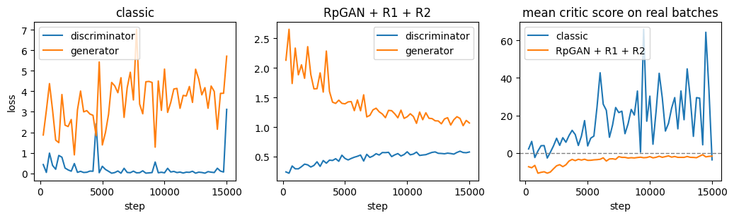
fig, axes = d2l.plt.subplots(1, 3, figsize=(10.5, 3.2))
for ax, (name, (ema_G, hist)) in zip(axes[:2], runs.items()):
    ax.plot(hist[:, 0], hist[:, 1], label='discriminator')
    ax.plot(hist[:, 0], hist[:, 2], label='generator')
    ax.set_title(name), ax.set_xlabel('step'), ax.legend()
axes[0].set_ylabel('loss')
for name, (ema_G, hist) in runs.items():
    axes[2].plot(hist[:, 0], hist[:, 3], label=name)
axes[2].axhline(0, ls='--', c='gray', lw=1)
axes[2].set_title('mean critic score on real batches')
axes[2].set_xlabel('step'), axes[2].legend()
fig.tight_layout()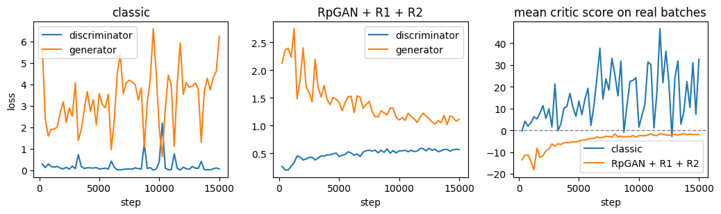
In the classic arm, the discriminator loss remains near zero while the generator loss is both larger and highly variable. The third panel helps explain this behavior: the critic’s scores on real images grow without bound and oscillate widely. By contrast, the penalized critic’s scores remain bounded. The penalties in Equation 16.4.4 act on the input gradient \(\nabla_x D\), not on the score itself. The increasing score level therefore accompanies an increasingly steep critic rather than being penalized directly, and the resulting one-sided gradients lead the generator to collapse.
In the penalized arm, both losses remain near their equilibrium values. After an initial transient, the critic’s mean score on real images stays within a narrow band. The position of this band varies between runs because the pairing objective depends only on score differences. Its absolute level is the shift-invariant direction identified in Section 16.3, and gradient penalties do not determine that level.
16.5.3.1 Architectural Developments after DCGAN
The preceding comparison moves directly from the 2015 recipe to a 2024 backbone. During the intervening decade, many improvements to image GANs were architectural responses to specific training failures. The pattern predates DCGAN: the Laplacian-pyramid GAN split generation into stages at different scales (Denton et al. 2015), while DCGAN replaced those stages with a single convolutional network stabilized by normalization (Radford et al. 2015). Later methods addressed high-resolution instability, critic smoothness, long-range structure, and controllable synthesis in turn.
| Design | Problem addressed |
|---|---|
| Progressive growing (Karras et al. 2018) | Instability at high resolution: both networks start at \(4 \times 4\) and grow in lockstep, so the game is never played at a resolution before the coarser ones have settled. |
| Spectral normalization (Miyato et al. 2018) | An unboundedly steep critic: dividing each weight matrix by its largest singular value caps the critic’s Lipschitz constant by construction. |
| Self-attention (Zhang et al. 2019) | Missing long-range structure: convolutional networks process texture locally, so attention gives both networks image-wide receptive fields. |
| BigGAN (Brock et al. 2019) | Small-scale ceilings: large batches, wide networks, and a catalog of stabilizing tricks, with the paper reporting that collapse is delayed rather than removed. |
| StyleGAN (Karras et al. 2019) | Entangled latent factors: a mapping network and per-layer style modulation separate coarse attributes from fine detail. |
| StyleGAN2 (Karras, Laine, et al. 2020) | Droplet artifacts introduced by StyleGAN’s own normalization, which is replaced by weight demodulation. |
| StyleGAN3 (Karras et al. 2021) | Texture sticking to pixel coordinates, an aliasing artifact of the resampling stack, which is replaced by band-limited resampling. |
| Projected discriminators (Sauer et al. 2021) | Slow, unreliable critic learning: the discriminator evaluates frozen pretrained features instead of learning image statistics from scratch. |
The methods in the second column address two types of problem. Some impose architectural constraints on pathologies derived earlier in the chapter. Spectral normalization is the hard-constraint counterpart of the zero-centered penalties: it bounds the critic’s steepness throughout the input space rather than penalizing gradients at the data. Progressive growing does not make the high-resolution game convergent; it postpones that game until training has established a coarse representation. Other methods correct artifacts introduced by previous architectures. StyleGAN2 removes artifacts caused by StyleGAN’s normalization, and StyleGAN3 removes aliasing caused by its resampling stack. These components accumulate because each addresses a different failure.
R3GAN tests this distinction directly (Huang et al. 2024). It first replaces the objective with the pairing loss and both zero-centered penalties from Section 16.4. It then uses a modern convolutional backbone without progressive growing, spectral normalization, attention, style modulation, or pretrained features. On standard benchmarks, this simpler network matches or exceeds the performance of architectures that combine those devices. The smaller comparison above follows the same design. Together, the results suggest that many architectural stabilizers compensated for deficiencies in the training objective. Capacity scaling and attention may still be useful for representational reasons. Pretrained discriminators require a separate caution: ImageNet features in the critic can favor evaluation metrics computed from similar features, a dependence considered below.
16.5.4 Measuring Sample Quality
Sample grids reveal gross failures such as collapse, but they do not support systematic comparisons across checkpoints or hyperparameters. An implicit generator also provides no likelihood with which to rank such models. Instead, common metrics pass \(n\) real and \(n\) generated images through a fixed feature map \(\phi\) and compare the resulting feature distributions. The two metrics used here apply the chapter’s analytically tractable Wasserstein and MMD cases in this feature space.
The Fréchet inception distance (FID) of Heusel et al. (2017) fits one Gaussian to each feature distribution: \(\mathcal{N}(\mu_p, \Sigma_p)\) for real features and \(\mathcal{N}(\mu_q, \Sigma_q)\) for generated features. It reports the squared Wasserstein-2 distance between these Gaussians. This is the closed form deferred in Section 16.2, where the general \(W_2\) problem in Equation 29.4.19 had no explicit solution (Dowson and Landau 1982; Givens and Shortt 1984):
\[ \mathrm{FID} = \big\| \mu_p - \mu_q \big\|^2 + \operatorname{tr}\!\Big( \Sigma_p + \Sigma_q - 2 \big( \Sigma_p^{1/2}\, \Sigma_q\, \Sigma_p^{1/2} \big)^{1/2} \Big). \tag{16.5.2}\]
The commuting case makes the formula easy to interpret. If \(\Sigma_p\) and \(\Sigma_q\) commute, they share an eigenbasis. Let \(\lambda_i\) and \(\nu_i\) denote their eigenvalues in this basis. The matrix \(\Sigma_p^{1/2} \Sigma_q \Sigma_p^{1/2}\) then has eigenvalues \(\lambda_i \nu_i\), and the trace term becomes \(\sum_i (\sqrt{\lambda_i}-\sqrt{\nu_i})^2\). FID therefore adds the squared distance between the means to the squared differences between standard deviations along the shared principal axes. In one dimension, it reduces to \((\mu_p-\mu_q)^2+(\sigma_p-\sigma_q)^2\); Exercise 1 derives this expression from optimal transport. The cited results establish the non-commuting case. FID has two immediate limitations: the Gaussian approximation retains only the first two feature moments, and its plug-in estimate is biased for finite \(n\).
The kernel inception distance (KID) of Bińkowski et al. (2018) uses the chapter’s other closed form, the maximum mean discrepancy. Its population value is the kernel expression Equation 28.2.9, and KID reports the unbiased estimator of that quantity, the U-statistic that omits the diagonal self-similarity terms:
\[ \widehat{\mathrm{MMD}}^2 = \frac{1}{m(m-1)} \sum_{i \neq j} k(\phi_i, \phi_j) + \frac{1}{n(n-1)} \sum_{i \neq j} k(\phi'_i, \phi'_j) - \frac{2}{mn} \sum_{i,j} k(\phi_i, \phi'_j), \tag{16.5.3}\]
with real features \(\phi_i\), generated features \(\phi'_j\), and the polynomial kernel \(k(u, v) = (u^\top v / d + 1)^3\) in \(d\) feature dimensions. In Section 16.2, MMD had a closed form because the kernel was fixed in advance. KID instead applies a fixed polynomial kernel to learned image features, so its sensitivity is determined jointly by the feature network and the kernel. The newer CMMD metric changes both components, using CLIP embeddings instead of Inception features and a Gaussian RBF kernel instead of the polynomial kernel. The estimator again requires \(O(n^2)\) pairwise evaluations, which is manageable at the sample sizes used here. Its unbiasedness has an observable consequence: on two disjoint samples of real images, the U-statistic fluctuates around zero and may be slightly negative. FID between the same finite samples remains positive because their fitted moments are not identical.
def fid_score(feat_p, feat_q):
    feat_p, feat_q = np.float64(feat_p), np.float64(feat_q)
    mu_p, mu_q = feat_p.mean(0), feat_q.mean(0)
    C_p = np.cov(feat_p, rowvar=False)
    C_q = np.cov(feat_q, rowvar=False)
    lam, U = np.linalg.eigh(C_p)
    sqrt_C_p = (U * np.sqrt(np.maximum(lam, 0))) @ U.T
    M = sqrt_C_p @ C_q @ sqrt_C_p
    cross = np.linalg.eigvalsh((M + M.T) / 2)   # symmetric up to rounding
    return (((mu_p - mu_q) ** 2).sum() + np.trace(C_p) + np.trace(C_q)
            - 2 * np.sqrt(np.maximum(cross, 0)).sum())

def kid_score(feat_p, feat_q):
    m, n, d = len(feat_p), len(feat_q), feat_p.shape[1]
    K_pp = (feat_p @ feat_p.T / d + 1) ** 3
    K_qq = (feat_q @ feat_q.T / d + 1) ** 3
    K_pq = (feat_p @ feat_q.T / d + 1) ** 3
    return ((K_pp.sum() - np.trace(K_pp)) / (m * (m - 1))
            + (K_qq.sum() - np.trace(K_qq)) / (n * (n - 1))
            - 2 * K_pq.mean())
def fid_score(feat_p, feat_q):
feat_p, feat_q = np.float64(feat_p), np.float64(feat_q)
mu_p, mu_q = feat_p.mean(0), feat_q.mean(0)
C_p = np.cov(feat_p, rowvar=False)
C_q = np.cov(feat_q, rowvar=False)
lam, U = np.linalg.eigh(C_p)
sqrt_C_p = (U * np.sqrt(np.maximum(lam, 0))) @ U.T
M = sqrt_C_p @ C_q @ sqrt_C_p
cross = np.linalg.eigvalsh((M + M.T) / 2) # symmetric up to rounding
return (((mu_p - mu_q) ** 2).sum() + np.trace(C_p) + np.trace(C_q)
- 2 * np.sqrt(np.maximum(cross, 0)).sum())
def kid_score(feat_p, feat_q):
m, n, d = len(feat_p), len(feat_q), feat_p.shape[1]
K_pp = (feat_p @ feat_p.T / d + 1) ** 3
K_qq = (feat_q @ feat_q.T / d + 1) ** 3
K_pq = (feat_p @ feat_q.T / d + 1) ** 3
return ((K_pp.sum() - np.trace(K_pp)) / (m * (m - 1))
+ (K_qq.sum() - np.trace(K_qq)) / (n * (n - 1))
- 2 * K_pq.mean())16.5.4.1 A Feature Network Trained in the Notebook
Both metrics require a feature map \(\phi\). Published FID usually uses pooled features from an Inception-v3 classifier trained on ImageNet. To keep the experiment reproducible within the notebook, we train a small convolutional classifier on CIFAR-10 in about two minutes and use its 128-dimensional penultimate layer as \(\phi\). This choice retains a limitation of standard FID: features learned on one distribution, here natural photographs from ten classes, evaluate another distribution, here sprites. We train the network on bilinearly upsampled \(64 \times 64\) CIFAR-10 images rather than downsampling the sprites to \(32 \times 32\). Downsampling generated images could suppress checkerboard texture and lost fine detail that the metric should detect.
d2l.DATA_HUB['cifar10'] = (
    'https://www.cs.toronto.edu/~kriz/cifar-10-python.tar.gz',
    '874905e36347c8536514d0a26261acf3bff89bc7')
cifar_dir = d2l.download_extract('cifar10', 'cifar-10-batches-py')

def load_cifar_batch(path):
    with open(path, 'rb') as f, warnings.catch_warnings():
        warnings.simplefilter('ignore')   # legacy NumPy pickle format
        batch = pickle.load(f, encoding='bytes')
    X = torch.tensor(batch[b'data'], dtype=torch.float32)
    return X.reshape(-1, 3, 32, 32) / 127.5 - 1, torch.tensor(
        batch[b'labels'])

Xs, ys = zip(*[load_cifar_batch(f'{cifar_dir}/data_batch_{i}')
               for i in range(1, 6)])
cifar_X, cifar_y = torch.cat(Xs).to(device), torch.cat(ys).to(device)
test_X, test_y = load_cifar_batch(f'{cifar_dir}/test_batch')
test_X, test_y = test_X.to(device), test_y.to(device)d2l.DATA_HUB['cifar10'] = (
'https://www.cs.toronto.edu/~kriz/cifar-10-python.tar.gz',
'874905e36347c8536514d0a26261acf3bff89bc7')
cifar_dir = d2l.download_extract('cifar10', 'cifar-10-batches-py')
def load_cifar_batch(path):
with open(path, 'rb') as f, warnings.catch_warnings():
warnings.simplefilter('ignore') # legacy NumPy pickle format
batch = pickle.load(f, encoding='bytes')
X = batch[b'data'].reshape(-1, 3, 32, 32).transpose(0, 2, 3, 1)
return (jnp.asarray(X, dtype=jnp.float32) / 127.5 - 1,
jnp.asarray(batch[b'labels']))
Xs, ys = zip(*[load_cifar_batch(f'{cifar_dir}/data_batch_{i}')
for i in range(1, 6)])
cifar_X, cifar_y = jnp.concatenate(Xs), jnp.concatenate(ys)
test_X, test_y = load_cifar_batch(f'{cifar_dir}/test_batch')class FeatureCNN(nn.Module):
"""Three conv blocks, global average pooling, and a linear head."""
def __init__(self, feature_dim=128):
super().__init__()
widths = [3, 32, 64, feature_dim]
self.blocks = nn.ModuleList(
[nn.Sequential(nn.Conv2d(c_in, c_out, 3, padding=1),
nn.BatchNorm2d(c_out), nn.ReLU(),
nn.MaxPool2d(2))
for c_in, c_out in zip(widths[:-1], widths[1:])])
self.head = nn.Linear(feature_dim, 10)
def features(self, x):
for block in self.blocks:
x = block(x)
return x.mean(dim=(2, 3))
def forward(self, x):
return self.head(self.features(x))
def upsample(X):
return F.interpolate(X, size=(64, 64), mode='bilinear')
torch.manual_seed(0)
cnn = FeatureCNN().to(device)
opt = torch.optim.Adam(cnn.parameters(), lr=0.001)
for epoch in range(3):
order = torch.randperm(len(cifar_X), device=device)
for i in range(0, len(order) - 255, 256):
idx = order[i:i + 256]
l = F.cross_entropy(cnn(upsample(cifar_X[idx])), cifar_y[idx])
opt.zero_grad(), l.backward(), opt.step()
cnn.eval()
with torch.no_grad():
pred = torch.cat([cnn(upsample(test_X[i:i + 1000])).argmax(1)
for i in range(0, len(test_X), 1000)])
print(f'CIFAR-10 test accuracy: {float((pred == test_y).float().mean()):.3f}')CIFAR-10 test accuracy: 0.552class FeatureCNN(nnx.Module):
"""Three conv blocks, global average pooling, and a linear head."""
def __init__(self, feature_dim=128, rngs=None):
rngs = nnx.Rngs(d2l.get_key()) if rngs is None else rngs
widths = [3, 32, 64, feature_dim]
self.convs = nnx.List(
[nnx.Conv(c_in, c_out, (3, 3), padding='SAME', rngs=rngs)
for c_in, c_out in zip(widths[:-1], widths[1:])])
self.norms = nnx.List([nnx.BatchNorm(c, rngs=rngs)
for c in widths[1:]])
self.head = nnx.Linear(feature_dim, 10, rngs=rngs)
def features(self, x):
for conv, norm in zip(self.convs, self.norms):
x = nnx.max_pool(nnx.relu(norm(conv(x))),
window_shape=(2, 2), strides=(2, 2))
return x.mean(axis=(1, 2))
def __call__(self, x):
return self.head(self.features(x))
def upsample(X):
return jax.image.resize(X, (X.shape[0], 64, 64, 3), method='bilinear')
@nnx.jit
def cnn_step(cnn, opt, X, y):
def loss_fn(cnn):
return optax.softmax_cross_entropy_with_integer_labels(
cnn(upsample(X)), y).mean()
l, grads = nnx.value_and_grad(loss_fn)(cnn)
opt.update(cnn, grads)
return l
cnn = FeatureCNN(rngs=nnx.Rngs(0))
opt = nnx.Optimizer(cnn, optax.adam(0.001), wrt=nnx.Param)
key = jax.random.PRNGKey(3)
for epoch in range(3):
key, kp = jax.random.split(key)
order = jax.random.permutation(kp, len(cifar_X))
for i in range(0, len(order) - 255, 256):
idx = order[i:i + 256]
cnn_step(cnn, opt, cifar_X[idx], cifar_y[idx])
cnn.eval()
pred = jnp.concatenate([cnn(upsample(test_X[i:i + 1000])).argmax(1)
for i in range(0, len(test_X), 1000)])
print(f'CIFAR-10 test accuracy: {float((pred == test_y).mean()):.3f}')CIFAR-10 test accuracy: 0.497The classifier’s accuracy is modest. It is sufficient for this experiment only if its learned features respond meaningfully to image structure; the limitations of this choice are examined below.
16.5.4.2 Scoring the Two Runs
We first estimate a finite-sample reference by comparing two disjoint sets of 500 real training images. Any nonzero distance between them reflects estimator noise and, for FD, finite-sample bias. We then compare 500 EMA samples from each training arm with 500 held-out real images. Because the feature network is trained within the chapter, the cells report FD (CIFAR-CNN) and MMD^2 (CIFAR-CNN). These use the same formulas as FID and KID but are not comparable with published Inception-based values. They are also not directly comparable between framework tabs because the two feature networks differ. A final column reports the fraction of raw generated pixels outside \([-1, 1]\). Evaluation clamps those values before scoring, so this fraction quantifies how much the scored distribution differs from the generator output seen by the critic.
def features(model, imgs, batch_size=250):
    with torch.no_grad():
        return np.concatenate(
            [model.features(imgs[i:i + batch_size]).cpu().numpy()
             for i in range(0, len(imgs), batch_size)])

n = 500
torch.manual_seed(7)
z_score = torch.randn(n, 100, device=device)
feat_real = features(cnn, holdout_imgs[:n])
floor_fd = fid_score(features(cnn, train_imgs[:n]),
                     features(cnn, train_imgs[n:2 * n]))
floor_mmd = kid_score(features(cnn, train_imgs[:n]),
                      features(cnn, train_imgs[n:2 * n]))
print(f'{"run":22s}{"FD (CIFAR-CNN)":>16s}{"MMD^2 (CIFAR-CNN)":>19s}'
      f'{"out-of-range":>14s}')
print(f'{"real vs. real":22s}{floor_fd:16.2f}{floor_mmd:19.2f}{"--":>14s}')
for name, (ema_G, hist) in runs.items():
    with torch.no_grad():
        raw = ema_G(z_score)
    oob = float(((raw < -1) | (raw > 1)).float().mean())
    feat = features(cnn, raw.clamp(-1, 1))
    print(f'{name:22s}{fid_score(feat, feat_real):16.2f}'
          f'{kid_score(feat, feat_real):19.2f}{oob:14.3f}')
run FD (CIFAR-CNN) MMD^2 (CIFAR-CNN) out-of-range
real vs. real 0.69 0.06 --
classic 179.51 125.83 0.000
RpGAN + R1 + R2 4.12 4.27 0.180def features(model, imgs, batch_size=250):
return np.concatenate(
[np.asarray(model.features(imgs[i:i + batch_size]))
for i in range(0, len(imgs), batch_size)])
n = 500
z_score = jax.random.normal(jax.random.PRNGKey(7), (n, 100))
feat_real = features(cnn, holdout_imgs[:n])
floor_fd = fid_score(features(cnn, train_imgs[:n]),
features(cnn, train_imgs[n:2 * n]))
floor_mmd = kid_score(features(cnn, train_imgs[:n]),
features(cnn, train_imgs[n:2 * n]))
print(f'{"run":22s}{"FD (CIFAR-CNN)":>16s}{"MMD^2 (CIFAR-CNN)":>19s}'
f'{"out-of-range":>14s}')
print(f'{"real vs. real":22s}{floor_fd:16.2f}{floor_mmd:19.2f}{"--":>14s}')
for name, (ema_G, hist) in runs.items():
raw = ema_G(z_score)
oob = float(((raw < -1) | (raw > 1)).mean())
feat = features(cnn, jnp.clip(raw, -1, 1))
print(f'{name:22s}{fid_score(feat, feat_real):16.2f}'
f'{kid_score(feat, feat_real):19.2f}{oob:14.3f}')run FD (CIFAR-CNN) MMD^2 (CIFAR-CNN) out-of-range
real vs. real 0.53 0.03 --
classic 104.05 26.99 0.000
RpGAN + R1 + R2 2.50 0.67 0.157Both scores rank the penalized relativistic run far above the collapsed classic run. The gap between the arms is two orders of magnitude larger than the real-versus-real reference, so estimator noise at this scale is unlikely to reverse the ordering. The numerical values remain specific to this run and feature network, but reruns with different feature-network seeds and larger sample sizes preserve the ordering. The reference row also demonstrates the finite-sample behavior described above: real-versus-real FD is positive because the fitted moments of two finite samples differ, whereas the unbiased \(\mathrm{MMD}^2\) estimate fluctuates around zero.
The main limitations concern the evaluation design. First, each score depends on the feature network as well as the generator. Our CIFAR-trained CNN emphasizes properties useful for CIFAR-10 classification, just as Inception features emphasize properties useful for ImageNet classification. Changing the feature network changes the values and may reverse the ordering of two similar models; Exercise 3 tests this dependence.
Second, the evaluation features may overlap with features used during training. Matching the ImageNet class histogram of the real data can reduce Inception-based FID without a visible improvement in sample quality. A discriminator built from ImageNet-pretrained features may exploit this dependence (Kynkäänniemi et al. 2023); R3GAN therefore reports results without pretrained discriminators (Huang et al. 2024). Third, preprocessing affects the score. Incorrect antialiasing during resizing can shift FID by amounts comparable to reported differences between methods (Parmar et al. 2022). We avoid one such change by training the feature network at the sprites’ native resolution. Finally, the finite-sample bias shown by the reference row depends on both the model and \(n\). At small sample sizes, this bias alone can reverse a ranking (Chong and Forsyth 2020); Exercise 2 measures the effect.
A single score also combines two distinct failures: low-fidelity samples and missing modes. The precision and recall metrics of Kynkäänniemi et al. (2019) separate them through feature-space neighborhoods. Precision measures the fraction of generated samples that lie within the support of the real features; recall measures the fraction of real samples covered by generated features. A collapsed generator can retain nonzero precision if its single output lies near the data manifold, while its recall approaches zero. FID does not expose this asymmetry. R3GAN therefore reports recall as a separate measure of diversity alongside FID.
16.5.5 Limited Data, Scale, and Scope
16.5.5.1 Training on Limited Data
Forty thousand sprites is a small dataset for a critic with 1.6 million parameters. During 15,000 steps at batch size 64, the critic sees each training image about twenty-five times on average. Rather than approximating a density ratio, it can begin to recognize individual training images. An overfit critic assigns higher scores to training images than to held-out real images. Its generator update then favors resemblance to a finite training set rather than the broader data distribution, and sample quality may decline. The A/B experiment therefore records the critic’s train–holdout score gap. This gap is near zero for the penalized arm on the present dataset. As the dataset shrinks, a fixed-capacity critic can separate training images from the rest of image space sooner, so the gap becomes an informative diagnostic (Karras, Aittala, et al. 2020).
Augmentation reduces critic memorization, but its placement determines the target distribution. Our loop flips only real images, treating the sprite distribution as approximately invariant to horizontal reflection. The plausibility of individual mirrored sprites alone would not establish exact invariance. Color jitter or cutout does not generally preserve that distribution. If these transformations are applied only to real images, the generator is trained to reproduce the transformed distribution and may generate color shifts or erased regions.
Differentiable augmentation instead applies the same random transformation to real and generated inputs during both updates (Zhao et al. 2020). The transformation remains in the generator’s differentiation path. Because the critic observes multiple transformed versions of each training image, direct memorization becomes harder. Applying the transformation to both distributions preserves the original matching problem when the transformation cannot map distinct distributions to the same one. Karras, Aittala, et al. (2020) call this requirement non-leaking.
The augmentation strength must also be controlled. Too little augmentation permits memorization, whereas too much makes the classification problem unnecessarily difficult. Adaptive discriminator augmentation changes the augmentation probability in response to an overfitting statistic (Karras, Aittala, et al. 2020). The authors considered the train–validation score gap used here, but adopted a related statistic computed from training images alone so that no data need be withheld. With this control, StyleGAN2 attains competitive quality on datasets of a few thousand images, about an order of magnitude smaller than its usual training sets.
Critic memorization and generator memorization require different diagnostics. To test the generator directly, we embed the same 500 generated samples used above in the CIFAR-CNN feature space and find each sample’s nearest training image. We calibrate these distances by matching held-out sprites against the same training set. A generator that copies its training data should place generated samples closer to individual training images than genuine held-out images are. Because variants of the same species may occur in both data splits, some held-out sprites already have close training neighbors. This makes the comparison conservative: it will detect pronounced copying but may miss more subtle reuse.
ema_G = runs['RpGAN + R1 + R2'][0]
with torch.no_grad():
    gen = ema_G(z_score).clamp(-1, 1)
feat_train_all = features(cnn, train_imgs)

def nearest_train(feat):
    d2 = ((feat ** 2).sum(1, keepdims=True) - 2 * feat @ feat_train_all.T
          + (feat_train_all ** 2).sum(1))
    return d2.argmin(1), np.sqrt(np.maximum(d2.min(1), 0))

nn_idx, d_gen = nearest_train(features(cnn, gen))
_, d_holdout = nearest_train(feat_real)
print(f'median distance to nearest training image: '
      f'generated {np.median(d_gen):.2f}, '
      f'held-out real {np.median(d_holdout):.2f}')
closest = np.argsort(d_gen)[:8]
pairs = torch.cat([gen[torch.as_tensor(closest, device=device)],
                   train_imgs[torch.as_tensor(nn_idx[closest],
                                              device=device)]])
d2l.show_images(pairs.cpu().permute(0, 2, 3, 1) / 2 + 0.5,
                num_rows=2, num_cols=8);
median distance to nearest training image: generated 2.42, held-out real 0.91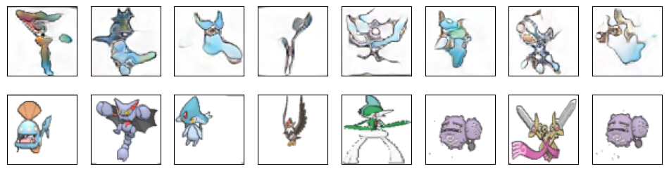
ema_G = runs['RpGAN + R1 + R2'][0]
gen = jnp.clip(ema_G(z_score), -1, 1)
feat_train_all = features(cnn, train_imgs)

def nearest_train(feat):
    d2 = ((feat ** 2).sum(1, keepdims=True) - 2 * feat @ feat_train_all.T
          + (feat_train_all ** 2).sum(1))
    return d2.argmin(1), np.sqrt(np.maximum(d2.min(1), 0))

nn_idx, d_gen = nearest_train(features(cnn, gen))
_, d_holdout = nearest_train(feat_real)
print(f'median distance to nearest training image: '
      f'generated {np.median(d_gen):.2f}, '
      f'held-out real {np.median(d_holdout):.2f}')
closest = np.argsort(d_gen)[:8]
pairs = jnp.concatenate([gen[closest], train_imgs[nn_idx[closest]]])
d2l.show_images(np.asarray(pairs) / 2 + 0.5, num_rows=2, num_cols=8);
median distance to nearest training image: generated 1.99, held-out real 0.68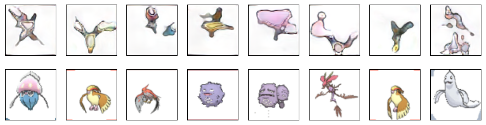
The generated samples are farther from the training set than the held-out sprites are, by a factor of two to three in the recorded runs. Copying would instead drive the generated distances toward zero. The lower held-out distances are consistent with the data split: many held-out sprites have a variant of the same species in the training set. The grid gives an image-level comparison. Its top row contains the eight generated samples closest to the training set, and its bottom row contains their nearest neighbors. Even these pairs depict different creatures; they share palettes or coarse silhouettes, but the generated samples are softer and less articulated.
This test has two limitations. Distances are defined by the CIFAR-CNN features, so they can detect direct copying but cannot rule out recombination of memorized parts. The result also applies only to this generator and dataset. Repeating the diagnostic after reducing the training set would reveal whether the generator begins to memorize under greater data scarcity. Exercise 6 extends the comparison to mirrored candidates and raw pixels.
16.5.5.2 Scale
The sprite experiment uses far less computation than published large-scale results, and the R3GAN paper provides useful reference budgets. StackedMNIST took 7 hours on eight L40 GPUs, CIFAR-10 four days on the same eight, FFHQ-256 about three weeks on eight A6000s, and conditional ImageNet about a day on 32 H100s (Huang et al. 2024). Our 15,000 steps on one GPU lie at the smallest end of a range spanning roughly four orders of magnitude.
Larger experiments require different schedules and numerical settings while using the same underlying objective and regularization. The penalty weight depends on resolution and dataset, ranging from 0.05 to 150 across R3GAN’s benchmarks compared with 10 here, and it is decayed together with the learning rate. R3GAN reports that mixed-precision training fails with FP16 and succeeds with BF16. The EMA half-life grows to millions of images and follows its own schedule, while the augmentation probability is tuned or controlled by feedback (Karras, Aittala, et al. 2020). These choices set the operating regime of the same method at larger scale.
The resulting image-generation pipeline specifies an objective, regularization, an architecture, and evaluation metrics. Each component follows from the analysis in Section 16.1 through Section 16.4. The next section adds conditional control through a class, caption, or source image. Chapter 17 covers diffusion models for large-scale image generation, Chapter 20 develops image-specific applications, and Section 16.7 examines adversarial losses within current systems.
16.5.6 Summary
Image generation requires both an architecture and an evaluation method. The 2015 DCGAN recipe improves the trainability of the classic objective through transposed convolutions, batch normalization, carefully chosen activations, and optimizer settings. A modern minimal backbone instead uses bilinear resampling, leaky ReLU, no normalization, and explicit latent injection.
On this backbone, the classic non-saturating loss collapses from the shared \(\mathcal{N}(0,0.02^2)\) initialization: every latent code maps to nearly the same image and the critic scores grow without bound. The same arm survives under the frameworks’ default initializations, showing that the failure depends on which initializations enter a mode-dropping basin. From the shared initialization, the relativistic pairing loss with both zero-centered penalties at \(\gamma=10\) trains stably and produces diverse sprites. The two-arm comparison changes the loss recipe as a whole; the component-wise evidence comes from Section 16.4 and the cited ablations. A feature-space nearest-neighbor check finds no evidence that the penalized generator copies training images.
We evaluate the runs with the Fréchet distance between Gaussian feature models and the unbiased MMD U-statistic. Because the feature network is trained within the chapter, the reported FD and \(\mathrm{MMD}^2\) values are not comparable with published Inception-based scores. Both metrics strongly prefer the penalized run, but their interpretation depends on the feature network, preprocessing, and sample size. On limited data, augmentation reduces critic memorization; applying the same differentiable transformation to real and generated inputs avoids changing the target distribution. Larger experiments alter the penalty schedule, EMA horizon, augmentation strength, and numerical precision, but use the same underlying method. Section 16.6 next introduces control through labels, text, or source images.
16.5.7 Exercises
- In one dimension, the squared Wasserstein-2 distance between distributions with quantile functions \(F^{-1}\) and \(G^{-1}\) is \(\int_0^1 \big(F^{-1}(u) - G^{-1}(u)\big)^2\, du\). Using the Gaussian quantile function \(F^{-1}(u) = \mu + \sigma\, \Phi^{-1}(u)\), show that for two univariate Gaussians this equals \((\mu_p - \mu_q)^2 + (\sigma_p - \sigma_q)^2\). Then verify that the multivariate formula Equation 16.5.2 reduces to a sum of such terms when \(\Sigma_p\) and \(\Sigma_q\) commute.
- Measure the finite-sample bias of FID directly: split the held-out sprites into two disjoint subsets of size \(n\) each and compute the real-versus-real FID and KID for \(n \in \{100, 250, 500, 2000\}\). How does each floor move with \(n\)? Now plot the FID estimates against \(1/n\) and extrapolate the fitted line to \(1/n \to 0\); this extrapolation is the bias-corrected estimator of Chong and Forsyth (2020) . How close is the extrapolated floor to zero, and what does the slope of the line say about the bias at \(n = 500\), the sample size this section uses?
- Retrain the feature network of this section on Fashion-MNIST instead of CIFAR-10 (replicate the grayscale channel three times, and upsample to \(64 \times 64\) as before), and rescore both arms. Do the FID and KID values change substantially? Does the ordering of the two arms change? Formulate in one sentence what this implies about comparing FID numbers computed with different feature networks.
- Apply the modern recipe to Fashion-MNIST: adapt the backbone to single-channel images (for instance by padding to \(32 \times 32\) and removing one upsampling stage), train once with the classic loss and once with the RpGAN plus \(R_1 + R_2\) loss at the same budget, and compare sample grids. Which of this section’s findings reproduce on a dataset with ten well-separated modes?
- Rerun arm A, the classic loss on the modern backbone, with the explicit \(\mathcal{N}(0, 0.02^2)\) initialization removed, so that your framework’s default initialization applies, keeping the architecture, optimizer, and budget fixed. Compare the resulting grid with the two grids of this section, and reconcile what you find with the landscape discussion of Section 16.3: the mode-dropping minima do not move when the initialization changes, so what does the outcome say about which starting points descend into them?
- Extend the memorization check of Section 16.5.5.1 in two directions. First, training presented every real image under a random horizontal flip, so a generator could reproduce the mirrored version of a training sprite, which a search over the stored images would miss: repeat the search with each training image and its mirror image both admitted as candidates, and report whether the distance distributions or the closest pairs change. Second, run the check in pixel space: use Euclidean distance between the flattened \(64 \times 64 \times 3\) images in place of feature distance, and display the ten closest pairs it finds. Compare the neighbors the two distances select. Which search is the stronger screen for copying, and why is near-duplicate detection usually run in a feature space rather than on raw pixels?