from d2l import torch as d2l
import numpy as np15.7 Reinforcement Learning for Sequence Generation
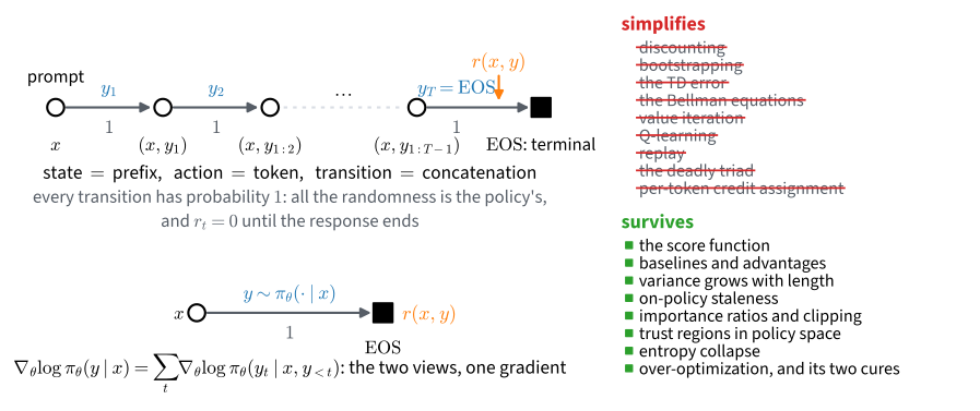
Autoregressive sequence generation can be written as a Markov decision process. The prompt is the start state, each token is an action, the prefix is the current state, and appending a token is a deterministic transition. A response is therefore a trajectory generated by the model’s next-token policy.
This special structure simplifies several reinforcement-learning methods. We prove that response-level and token-level score-function gradients are equivalent, identify which components of the preceding chapters remain useful under terminal rewards and deterministic transitions, and study group baselines and KL regularization in a small language-model example. The resulting notation is used later in the Language Models part.
from d2l import jax as d2l
import numpy as np
15.7.1 Text Generation as a Markov Decision Process
15.7.1.1 Prompt, Token, Prefix and Response
A language model with parameters \(\theta\) maps a context to a distribution over the next token through the softmax head of Section 11.2. The generation loop samples a token, appends it to the context, and stops at EOS (Section 8.7). Interpreting the context as a state and the token as an action gives the correspondence in Table 15.7.1.
| language modeling | reinforcement learning |
|---|---|
| prompt \(x\) | start state \(s_0\), drawn from the prompt distribution \(\mu_0\) of Section 14.1 |
| token \(y_t\) | action \(a_t\) |
| prefix \((x, y_{<t})\) | state \(s_t\) |
| response \(y = (y_1, \ldots, y_T)\) | trajectory \(\tau\) |
| EOS | terminal state |
| the next-token softmax of Section 11.2 | the policy \(\pi_\theta(a \mid s)\) of Section 14.5 |
the generate loop of Section 8.7 |
the rollout of Section 14.5 |
The state is the complete prefix, not only the last token. Conditional on that prefix, deterministic concatenation and the next-token policy specify the distribution of the next prefix, so the representation is Markov.
The start-state distribution \(\mu_0\) is the distribution over prompts. It does not depend on \(\theta\) and therefore contributes no score term to the policy-gradient derivation. It nevertheless determines which prompts and responses the objective weights, so empirical conclusions remain specific to the chosen prompt distribution.
15.7.1.2 Deterministic Transitions
The transition kernel is string concatenation: from prefix \(s_t\) and token \(a_t\), the next state is \((s_t, a_t)\) with probability one. A terminal reward \(r(x,y)\) is assigned when the response ends. This is the deterministic case described in Section 14.1. In Section 14.5, the trajectory probability Equation 14.5.3 includes transition factors; here each factor is the constant one and contributes no score term. Under these assumptions, all rollout randomness comes from policy sampling. Unlike the model-free setting in Section 14.4, the transition model is known exactly.
15.7.1.3 The Factorization Proposition
The following identity connects a response distribution to its next-token factorization.
Proposition. For the token MDP of Table 15.7.1, the response-level and token-level views give the same gradient:
\[\nabla_\theta \log \pi_\theta(y \mid x) = \sum_{t=1}^{T} \nabla_\theta \log \pi_\theta(y_t \mid x, y_{<t}). \tag{15.7.1}\]
Moreover, with a terminal-only reward \(r(x, y)\) and no discounting, every reward-to-go in the response is the same number, so a single response-level weight \(r(x, y) - b(x)\) multiplies every token’s score, without bias for any baseline \(b\) that depends only on the prompt.
Proof. The chain rule of probability factorizes the response’s likelihood exactly, \(\pi_\theta(y \mid x) = \prod_{t=1}^{T} \pi_\theta(y_t \mid x, y_{<t})\), with no transition factors because the transitions are deterministic; taking logarithms and gradients gives Equation 15.7.1. With rewards zero until EOS and \(\gamma = 1\), the reward-to-go of Section 14.6 is \(\hat{G}_t = r(x, y)\) at every \(t\); subtracting a prompt-only baseline \(b(x)\) is licensed bias-free by the zero-mean lemma of Section 14.6, leaving the weight \(r(x, y) - b(x)\) on every score. \(\blacksquare\)
The left side of Equation 15.7.1 treats a complete response as one structured action, while the right side factorizes it into \(T\) next-token actions. Because the response log-probability is the sum of the token log-probabilities, REINFORCE gives the same gradient in either view.
The quantity \(r(x,y)-b(x)\) is a response-level Monte Carlo weight applied to every token score. It is not the token advantage \(A(s_t,a_t)=Q(s_t,a_t)-V(s_t)\), whose terms condition on each prefix and may differ across positions. A single terminal response score therefore does not provide within-response credit assignment.
Under these single-turn assumptions, the response-level problem is a contextual bandit: a prompt is sampled, one structured action is scored, and no action changes a future context. Multi-turn dialogue, tool use, and environment feedback restore controlled transitions and require the sequential formulation.
15.7.2 Simplifications for Sequence Generation
The correspondence in Table 15.7.1 determines which general reinforcement-learning components simplify; Figure 15.7.1 summarizes the result.
15.7.2.1 Terms That Disappear
Several parts of the general MDP formulation simplify under these assumptions. A finite response receives one terminal reward, so we use \(\gamma=1\). There is no intermediate target for TD learning, and neither Bellman backups nor value iteration are needed for the derivation below. The methods remain close to on-policy and therefore do not use Q-learning’s replay mechanism. Every token receives the same response-level reward, so the formulation does not solve within-response credit assignment. These simplifications depend on deterministic concatenation and a terminal reward in a single turn. Process rewards reintroduce intermediate credit, while tool calls, environment feedback, and multi-turn interaction restore nontrivial transitions.
15.7.2.2 The Remaining Optimization Problem
The policy-optimization components remain applicable: the score-function identity and REINFORCE; action-independent baselines defined per prompt; importance ratios and clipping for limited batch reuse; policy-space trust regions; entropy or reference-policy regularization; and safeguards against optimizing reward-model error. Sequence length still matters because Equation 15.7.1 sums \(T\) score terms, and an updated policy no longer matches responses sampled before the update.
By contrast, this terminal-reward derivation does not use a learned transition model, intermediate Bellman backups, or token-level TD targets. Those components return when the task supplies process rewards or nontrivial environment transitions.
15.7.2.3 The Smallest Instance: Four Prompts and a Verifier
We study a finite one-step example that requires no environment simulator. It contains four prompts, nine candidate responses shared across prompts, an exact-match verifier, and a reference policy \(\pi_{\textrm{ref}}\) representing a pretrained model. The reference assigns probability across the ordinary candidates and about \(0.2\) percent to a response that lists every possible answer. For two prompts, no individual candidate matches the answer, so the maximum exact-match score is \(0.5\). The policy is Equation 14.5.1, one preference row per prompt; training starts from the reference, as post-training does.
prompts = ['2+2', '3*4', '8*8', '9*9']     # four prompts
answers = ['4', '12', '64', '81']          # their checked answers
resp = ['1', '3', '4', '7', '12', '19', '23', '35',
        'one of 4, 12, 64 or 81']          # nine candidate responses

def verify(x, y):                          # the verifier: exact match
    return float(resp[y] == answers[x])

def policy(theta):                         # pi(y | x), one row per prompt
    z = np.exp(theta - theta.max(1, keepdims=True))
    return z / z.sum(1, keepdims=True)

def success(pi, reward):                   # E r(x, y) over sampled y
    R = [[reward(x, y) for y in range(len(resp))] for x in range(4)]
    return (pi * np.array(R)).sum(1).mean()

theta_ref = np.zeros((4, 9))
theta_ref[:, 8] = -4.0                     # the reference rarely hedges
pi_ref = policy(theta_ref)
print(f'success of a response sampled from the reference: '
      f'{success(pi_ref, verify):.3f}')
success of a response sampled from the reference: 0.062prompts = ['2+2', '3*4', '8*8', '9*9'] # four prompts
answers = ['4', '12', '64', '81'] # their checked answers
resp = ['1', '3', '4', '7', '12', '19', '23', '35',
'one of 4, 12, 64 or 81'] # nine candidate responses
def verify(x, y): # the verifier: exact match
return float(resp[y] == answers[x])
def policy(theta): # pi(y | x), one row per prompt
z = np.exp(theta - theta.max(1, keepdims=True))
return z / z.sum(1, keepdims=True)
def success(pi, reward): # E r(x, y) over sampled y
R = [[reward(x, y) for y in range(len(resp))] for x in range(4)]
return (pi * np.array(R)).sum(1).mean()
theta_ref = np.zeros((4, 9))
theta_ref[:, 8] = -4.0 # the reference rarely hedges
pi_ref = policy(theta_ref)
print(f'success of a response sampled from the reference: '
f'{success(pi_ref, verify):.3f}')success of a response sampled from the reference: 0.06215.7.2.4 The Group Mean as the Baseline
For each prompt, we sample a group of \(K\) responses, score them, standardize scores within the group, and take one ascent step on the log-probabilities. This applies Equation 14.6.11 with the group as the batch and the prompt as the start state. The group mean serves as a per-prompt baseline, so the example uses no value network. We also include the fixed-reference KL penalty from Section 15.3 by replacing each sampled reward with \(r - \beta \log \big( \pi_\theta(y \mid x) / \pi_{\textrm{ref}}(y \mid x) \big)\). The GRPO objective described below instead estimates KL as a separate loss term. Setting \(\beta=0\) removes this penalty.
def group_step(theta, K, reward, rng, beta=0.0, lr=2.0):
    pi, g = policy(theta), np.zeros_like(theta)
    for x in range(len(prompts)):              # one group of K per prompt
        ys = rng.choice(len(resp), K, p=pi[x])
        r = np.array([reward(x, y) for y in ys])
        r = r - beta * np.log(pi[x, ys] / pi_ref[x, ys])   # the KL penalty
        A = d2l.normalize(r)                   # the group mean as baseline
        g[x] = (np.eye(len(resp))[ys] - pi[x]).T @ A / K   # eq_softmax_score
    return theta + lr * g
def group_step(theta, K, reward, rng, beta=0.0, lr=2.0):
pi, g = policy(theta), np.zeros_like(theta)
for x in range(len(prompts)): # one group of K per prompt
ys = rng.choice(len(resp), K, p=pi[x])
r = np.array([reward(x, y) for y in ys])
r = r - beta * np.log(pi[x, ys] / pi_ref[x, ys]) # the KL penalty
A = d2l.normalize(r) # the group mean as baseline
g[x] = (np.eye(len(resp))[ys] - pi[x]).T @ A / K # eq_softmax_score
return theta + lr * gThe zero-mean lemma applies only when a baseline does not depend on the sampled action. A same-group mean includes the current sample’s reward, so centering by it produces a biased estimator whose expectation is \((K-1)/K\) times the true gradient, as derived in Section 14.6. The leave-one-out correction is also described in Section 14.6. Division by the group standard deviation adds a random scale factor. Leave-one-out centering is unbiased because each sample is compared with the mean of the other \(K-1\) samples. The following enumeration verifies the centering result for groups of two, without standardization:
K, pi = 2, policy(theta_ref)
Rv = np.array([[verify(x, y) for y in range(len(resp))] for x in range(4)])
S = np.eye(len(resp))[None, :, :] - pi[:, None, :]   # eq_softmax_score
g = np.einsum('xy,xy,xyv->xv', pi, Rv, S)            # the exact gradient
u = np.zeros_like(g)
for y1, y2 in np.ndindex(len(resp), len(resp)):      # every group of K = 2
    w = (Rv[:, y1] - Rv[:, y2]) / 2                  # reward minus group mean
    u += (pi[:, y1] * pi[:, y2] * w)[:, None] * (S[:, y1] - S[:, y2]) / K
print(f'E of the group-centered update is (K-1)/K of the gradient: '
      f'{np.allclose(u, g * (K - 1) / K)}')
print(f'rescaled by K/(K-1), leave-one-out, it is exact: '
      f'{np.allclose(u * K / (K - 1), g)}')
E of the group-centered update is (K-1)/K of the gradient: True
rescaled by K/(K-1), leave-one-out, it is exact: TrueK, pi = 2, policy(theta_ref)
Rv = np.array([[verify(x, y) for y in range(len(resp))] for x in range(4)])
S = np.eye(len(resp))[None, :, :] - pi[:, None, :] # eq_softmax_score
g = np.einsum('xy,xy,xyv->xv', pi, Rv, S) # the exact gradient
u = np.zeros_like(g)
for y1, y2 in np.ndindex(len(resp), len(resp)): # every group of K = 2
w = (Rv[:, y1] - Rv[:, y2]) / 2 # reward minus group mean
u += (pi[:, y1] * pi[:, y2] * w)[:, None] * (S[:, y1] - S[:, y2]) / K
print(f'E of the group-centered update is (K-1)/K of the gradient: '
f'{np.allclose(u, g * (K - 1) / K)}')
print(f'rescaled by K/(K-1), leave-one-out, it is exact: '
f'{np.allclose(u * K / (K - 1), g)}')E of the group-centered update is (K-1)/K of the gradient: True
rescaled by K/(K-1), leave-one-out, it is exact: TrueAt \(K=1\), the factor \((K-1)/K\) is zero: the group mean equals the sample’s reward, the standardized advantage is zero, and the reward-gradient update does not change the parameters. The underlying policy gradient is generally nonzero, and REINFORCE without this baseline would still learn. The \(K=1\) row below therefore retains the reference score of \(0.062\). The sweep fixes the sample budget at \(6400\) scored responses per prompt, so smaller groups receive proportionally more updates:
budget = 6400                    # scored responses per prompt, matched
for K in (1, 2, 4, 8, 32):
    rng, theta = np.random.default_rng(1), theta_ref.copy()
    for _ in range(budget // K):
        theta = group_step(theta, K, verify, rng)
    print(f'K = {K:2d}: success of a sampled response '
          f'{success(policy(theta), verify):.3f}')
K = 1: success of a sampled response 0.062
K = 2: success of a sampled response 0.500
K = 4: success of a sampled response 0.500
K = 8: success of a sampled response 0.500
K = 32: success of a sampled response 0.500budget = 6400 # scored responses per prompt, matched
for K in (1, 2, 4, 8, 32):
rng, theta = np.random.default_rng(1), theta_ref.copy()
for _ in range(budget // K):
theta = group_step(theta, K, verify, rng)
print(f'K = {K:2d}: success of a sampled response '
f'{success(policy(theta), verify):.3f}')K = 1: success of a sampled response 0.062
K = 2: success of a sampled response 0.500
K = 4: success of a sampled response 0.500
K = 8: success of a sampled response 0.500
K = 32: success of a sampled response 0.500The \(K=1\) result matches the predicted reference score to three decimal places, while every tested \(K\geq2\) reaches the verifier ceiling of \(0.5\) at the same sample budget. For \(K\geq2\), the factor \((K-1)/K\) rescales the centered gradient rather than eliminating it. The group samples provide the per-prompt comparison that a learned value baseline would otherwise supply, but the current sample’s inclusion causes the stated bias. If every response in a group receives the same score, all standardized advantages are zero; this occurs on prompts that the current policy always fails or always solves. The zero-update result is specific to the reward-gradient term. Separate KL gradients, supervised objectives, or other loss terms can still update parameters at \(K=1\).
15.7.3 Where the Reward Comes From
The preceding analysis concerned the policy estimator. In large-scale applications, the reward \(r(x,y)\) is typically learned from preferences or computed by a verifier.
15.7.3.1 Learned Rewards from Preferences
When quality cannot be computed directly, people can compare pairs of responses to the same prompt, and a reward model \(r_\phi(x,y)\) can be fitted with the Bradley-Terry model from Section 15.3, Equation 15.3.1. Its evidence is strongest on the distribution represented by preference data, and its score is identifiable only up to an additive function of the prompt. A per-prompt baseline removes this unidentified term. A response-level reward is also terminal, matching the assumptions of the factorization proposition.
15.7.3.2 Checked Rewards from Verifiers
For a growing family of tasks the reward needs no model at all, because the response can be checked: a unit-test harness runs the code, a proof assistant validates the derivation, an exact-match grader scores the final answer. Training against such checked rewards is called reinforcement learning from verifiable rewards, RLVR, the regime in which recent reasoning models are trained (DeepSeek-AI 2025). A verifier has a different error profile from a learned reward model: it is reliable for the property it checks but may omit relevant aspects of the intended objective.
15.7.3.3 Reward Hacking as One Mechanism
Both learned reward models and programmatic verifiers are estimates of the intended objective, and optimization can exploit their errors. This is the same mechanism seen for a fitted \(\hat{Q}\) in Section 15.6 and for a learned reward in Section 15.3. To demonstrate this mechanism, replace exact matching with a verifier that searches for the answer string. The response listing all answers then receives reward on every prompt, including the two without an individual correct candidate. Equation Equation 15.3.3 predicts the regularization required to suppress this response: its reference log-odds disadvantage is \(4\), while its reward advantage is \(1\), giving the threshold \(\beta=1/4\).
def sloppy(x, y):                  # accepts anything containing the answer
    return float(answers[x] in resp[y])

for beta in (0.0, 0.1, 0.2, 0.3, 0.5):
    rng, theta = np.random.default_rng(2), theta_ref.copy()
    for _ in range(400):
        theta = group_step(theta, 32, sloppy, rng, beta=beta)
    pi = policy(theta)
    print(f'beta = {beta:.1f}: sloppy {success(pi, sloppy):.2f}, '
          f'gold {success(pi, verify):.2f}, hedge {pi[:, 8].mean():.2f}')
beta = 0.0: sloppy 1.00, gold 0.50, hedge 0.50
beta = 0.1: sloppy 0.99, gold 0.50, hedge 0.49
beta = 0.2: sloppy 0.60, gold 0.48, hedge 0.12
beta = 0.3: sloppy 0.42, gold 0.39, hedge 0.04
beta = 0.5: sloppy 0.25, gold 0.24, hedge 0.01def sloppy(x, y): # accepts anything containing the answer
return float(answers[x] in resp[y])
for beta in (0.0, 0.1, 0.2, 0.3, 0.5):
rng, theta = np.random.default_rng(2), theta_ref.copy()
for _ in range(400):
theta = group_step(theta, 32, sloppy, rng, beta=beta)
pi = policy(theta)
print(f'beta = {beta:.1f}: sloppy {success(pi, sloppy):.2f}, '
f'gold {success(pi, verify):.2f}, hedge {pi[:, 8].mean():.2f}')beta = 0.0: sloppy 1.00, gold 0.50, hedge 0.50
beta = 0.1: sloppy 0.99, gold 0.50, hedge 0.49
beta = 0.2: sloppy 0.60, gold 0.48, hedge 0.12
beta = 0.3: sloppy 0.42, gold 0.39, hedge 0.04
beta = 0.5: sloppy 0.25, gold 0.24, hedge 0.01The columns report the approximate grader score, the exact score, and the average probability of the hedged response. At \(\beta=0\), the policy obtains a perfect grader score but only \(0.50\) under exact evaluation. The multi-answer response remains favored at \(\beta=0.1\), is nearly balanced at \(0.2\), and is suppressed above the predicted threshold of \(1/4\). Each row is close to the tilted optimum in Equation 15.3.3, although group standardization introduces a random denominator and can shift the stationary point. Larger \(\beta\) also limits useful changes to the policy: at \(\beta=0.5\), the exact score falls to \(0.24\). Thus regularization selects a point on the reward–divergence frontier rather than providing an absolute safeguard.
15.7.4 GRPO and the Notation Contract
15.7.4.1 Components of GRPO
Group Relative Policy Optimization (GRPO) (Shao et al. 2024) samples \(K\) responses for each prompt and uses the group-standardized response score
\[A_j=\frac{r_j-\mu}{\sigma+10^{-8}}\]
as the weight on every token of response \(j\). The group mean replaces a learned per-prompt value baseline, while division by \(\sigma\) rescales the update rather than providing an additional zero-mean control variate. Reusing a group for several epochs introduces token-level ratios \(\rho_t\) and the clipped objective Equation 15.2.10. A separate KL penalty anchors the policy to a frozen reference, and the cited loss normalizes each response by its length.
Two different reference policies appear. Clipping compares the current policy with the policy that sampled the batch and limits each update. The \(\beta\) penalty compares with a frozen reference and changes the optimum. They therefore play the two distinct roles described in Section 15.3.
The finite experiment above is not a complete GRPO implementation. It takes one update per group, folds the KL term into the reward, uses one-token responses, and applies no response-length normalization. It does share the same-group mean and hence the self-inclusion bias measured above; RLOO replaces that mean with the unbiased leave-one-out baseline from Section 14.6.
Direct Preference Optimization (DPO) uses a different objective. Solving Equation 15.3.3 for the reward gives
\[r(x,y)=\beta\log\frac{\pi^\star(y\mid x)} {\pi_{\textrm{ref}}(y\mid x)}+c(x), \tag{15.7.2}\]
where \(c(x)\) is unidentified by same-prompt comparisons. Substituting this relation into the preference likelihood fits the policy directly rather than first fitting a scalar reward model (Rafailov et al. 2023). The Language Models part develops that derivation and its assumptions.
15.7.4.2 Notation Inherited by the Language Models Part
The Language Models part inherits these symbols verbatim; every object below was defined and exercised in these two chapters.
| symbol | meaning | built in |
|---|---|---|
| \(x\), \(y\) | prompt, response | this section |
| \(\tau\) | trajectory | Section 14.1 |
| \(\mu_0\) | start-state, i.e. prompt, distribution | Section 14.1 |
| \(\pi_\theta\), \(\pi_{\textrm{ref}}\) | policy; frozen reference | Section 14.5, Section 15.3 |
| \(\hat{G}_t\) | reward-to-go | Section 14.6 |
| \(A\) | advantage | Section 14.2, Section 14.6 |
| \(K\) | group size | Section 14.6 |
| \(\rho_t\) | importance ratio \(\pi_\theta / \pi_{\theta_{\textrm{old}}}\) | Section 15.2 |
| \(\epsilon\) | clip half-width, exploration rate; never a numerical constant | Section 15.2, Section 14.4 |
| \(\beta\) | KL coefficient | Section 15.3 |
| \(\delta_t\) | TD error | Section 14.4 |
| \(w\), \(w^-\) | critic parameters; target copy | Section 15.1, Section 15.4 |
| \(D_{\textrm{KL}}(P \Vert Q)\), \(\mathbf{1}(\cdot)\) | KL divergence; indicator | Section 15.3 |
15.7.5 Where to Go Next
These chapters provide an introduction rather than comprehensive coverage. Three extensions are especially relevant.
Model-based reinforcement learning and search. Section 14.2 is the book’s only model-based method. A direct extension is Dyna-Q: augment Section 14.4’s tabular loop by storing observed transitions and applying the same Q-update to model-generated transitions between environment steps. Monte Carlo tree search can be viewed as a policy-improvement operator: search produces an improved action distribution, which is then distilled into the policy as a supervised target. That loop is AlphaZero (Silver et al. 2017, 2018); MuZero learns the model it searches in (Schrittwieser et al. 2020); DreamerV3 and TD-MPC2 train control inside learned world models (Hafner et al. 2025; Hansen et al. 2024). The same search-and-distillation pattern appears in test-time reasoning methods for language models.
Continuous control since 2024. The objectives of Section 14.7 through Section 15.3 stand; recent gains have come from normalization, scale and stability rather than new losses, and careful normalization even lets streaming, replay-free temporal-difference learning work after decades of not working (Elsayed et al. 2024; Gallici et al. 2025). Reading a modern paper here, you should recognize nearly every symbol.
What we deliberately left out. Multi-agent reinforcement learning, where the opponent learns too, reached superhuman poker with search plus self-play (Brown and Sandholm 2017). Distributional reinforcement learning models the return’s whole distribution rather than its mean (Bellemare et al. 2017). Meta-learning, hierarchy and partial observability each relax one of Section 14.1’s assumptions; Murphy’s overview treats all three at textbook depth (Murphy 2025). For a broader treatment of post-training practice, see the reinforcement-learning-from-human-feedback book (Lambert 2026).
15.7.6 Capstone Projects
These four projects play the role of a course programming assignment; each runs on a laptop CPU in minutes, and each carries a numeric sanity bar in place of an autograder.
A. Build PPO from the pieces, and prove it is right. Three self-checks: the ratio is exactly \(1\) on the first epoch; GAE at \(\lambda = 1\) equals reward-to-go minus \(\hat{V}\) to floating-point tolerance; the clipped objective’s gradient at \(\theta = \theta_{\textrm{old}}\) equals the plain policy gradient. Bar: median return above \(450\) on CartPole within \(60\) updates, 3 seeds.
B. Which implementation details actually matter. Ablate five of the 37 catalogued PPO details, one at a time, three seeds each. Bar: at least one factor changes the median by more than the seed spread, and you can say which.
C. Diagnose three faulty policies. Examine one agent with a saturated policy, one with an untrained critic, and one with an undersized replay buffer. Identify each fault from the chapter’s diagnostics before inspecting the code.
D. GRPO from REINFORCE, in two lines. Start from Section 14.6’s train, add the group-standardized weight and the clip, and reproduce this section’s \(K\)-sweep. Bar: \(K = 1\) shows no learning; \(K \geq 4\) reaches the verifier’s ceiling.
15.7.7 Summary
In sequence generation, prompts are start states, tokens are actions, prefixes are states, and responses are trajectories with deterministic concatenation transitions. The response probability factorizes into next-token probabilities, so the response-level score equals the sum of token-level scores. With terminal reward, every token receives the same response-level weight unless an additional credit-assignment model is introduced. A same-group mean baseline shrinks the expected gradient by \((K-1)/K\); leave-one-out centering removes this bias. Learned rewards and programmatic verifiers can both be misspecified, and a KL penalty relative to a reference policy limits the resulting policy shift.
Experimental scope. The examples use four prompts and finite response sets. The \(K=1\) same-group update is exactly zero, while all tested \(K\geq2\) solve this small problem. The verifier example uses a deliberately constructed loophole and a reference distribution chosen to give a threshold near \(\beta=1/4\). It illustrates the mechanism of reward exploitation, not the scale or complexity of language-model post-training.
15.7.8 Exercises
- [conceptual] The factorization. Prove \(\nabla_\theta \log \pi_\theta(y \mid x) = \sum_t \nabla_\theta \log \pi_\theta(y_t \mid x, y_{<t})\) and say why this makes the token-level and response-level views the same algorithm.
- [conceptual] Which terms disappear. For each of discounting, bootstrapping, the TD error and replay, say in one sentence what property of the token MDP removes it, and name one setting (multi-turn dialogue, tool use) in which it comes back.
- [short-code] Why \(K = 1\) learns nothing. Predict it from the \((K-1)/K\) shrinkage of Section 14.6, run it, and say why leave-one-out has no defined value at \(K = 1\).
- [short-code] Price the exploit. Find the \(\beta\) at which the KL penalty makes the verifier loophole unprofitable, and relate it to the reward gap between the exploit and the honest solution.
- [conceptual] Read a paper. Take the GRPO objective as published and name, for each symbol, the section of these two chapters that built it, and the one component that is not in these chapters at all.