%matplotlib inline
from d2l import torch as d2l
import gymnasium as gym
import numpy as np
import torch
from torch import nn
torch.set_num_threads(1)15.5 Soft Actor-Critic
Soft Actor-Critic (SAC) combines an entropy-regularized objective with off-policy value learning for continuous actions (Haarnoja, Zhou, Abbeel, et al. 2018; Haarnoja, Zhou, Hartikainen, et al. 2018). Its actor uses a pathwise gradient through a differentiable critic, while replay, target networks, and double critics stabilize value learning. Bounded actions are represented by applying a hyperbolic tangent to a Gaussian sample, which requires a change-of-variables correction to the log density.
This section derives the soft policy-evaluation and improvement steps, constructs the squashed Gaussian policy, and assembles the SAC update. On Pendulum, we compare sample efficiency with REINFORCE and evaluate both policy return and critic calibration.
%matplotlib inline
from d2l import jax as d2l
from flax import nnx
import gymnasium as gym
import jax
from jax import numpy as jnp
import numpy as np
import optax
Pendulum has state \((\cos\vartheta,\sin\vartheta,\dot\vartheta)\) and torque actions in \([-2,2]\). An uncontrolled policy obtains a return near \(-1200\), while a controller that swings up and balances obtains about \(-200\) or better. Each run uses \(20{,}000\) environment steps, with one gradient update per step after \(1{,}000\) random warm-up steps. Each critic takes a state and action as input and returns a scalar value; the actor replaces explicit maximization over continuous actions.
gamma, num_env_steps, num_seeds = 0.99, 20_000, 3
buffer_size, batch_size, lr = 200_000, 256, 3e-4
alpha, tau, warmup, c = 0.2, 0.005, 1_000, 2.0
if tab.selected('pytorch'):
    def make_critic():
        return nn.Sequential(nn.Linear(4, 64), nn.ReLU(),
                             nn.Linear(64, 64), nn.ReLU(),
                             nn.Linear(64, 1))
if tab.selected('jax'):
    def make_critic(rngs):
        return nnx.Sequential(nnx.Linear(4, 64, rngs=rngs), jax.nn.relu,
                              nnx.Linear(64, 64, rngs=rngs), jax.nn.relu,
                              nnx.Linear(64, 1, rngs=rngs))
gamma, num_env_steps, num_seeds = 0.99, 20_000, 3
buffer_size, batch_size, lr = 200_000, 256, 3e-4
alpha, tau, warmup, c = 0.2, 0.005, 1_000, 2.0
if tab.selected('pytorch'):
def make_critic():
return nn.Sequential(nn.Linear(4, 64), nn.ReLU(),
nn.Linear(64, 64), nn.ReLU(),
nn.Linear(64, 1))
if tab.selected('jax'):
def make_critic(rngs):
return nnx.Sequential(nnx.Linear(4, 64, rngs=rngs), jax.nn.relu,
nnx.Linear(64, 64, rngs=rngs), jax.nn.relu,
nnx.Linear(64, 1, rngs=rngs))15.5.1 The Objective and Its Two Backups
15.5.1.1 The Maximum-Entropy Objective
Section Section 15.3 derived an objective with a per-step KL penalty relative to a fixed reference policy. For a uniform reference, this penalty is equivalent to an entropy bonus up to a policy-independent constant. SAC maximizes this special case, conventionally writing \(\alpha\) for the coefficient denoted by \(\beta\) in Section 15.3:
\[ J(\pi) = E_{\pi}\Big[ \sum_t \gamma^t \big( r_t + \alpha\, H(\pi(\cdot \mid s_t)) \big) \Big]. \tag{15.5.1}\]
Unlike the optional entropy term in Section 15.2’s actor loss, the entropy term here is part of the objective and changes the optimum. The optimal policy can therefore remain stochastic after training. For continuous actions, this quantity is differential entropy, which is defined by an integral and can be negative. This distinction matters when interpreting the diagnostics below. This is maximum-entropy reinforcement learning, a line of work older than deep learning (Ziebart et al. 2008), read by Section 15.3 as inference (Levine 2018); SAC is its off-policy actor-critic instance, with a lineage running through soft Q-learning (Haarnoja et al. 2017).
Equation Equation 15.5.1 can be optimized by generalized policy iteration (Figure 14.2.3): policy evaluation estimates values under the current policy, and policy improvement updates the policy using those estimates. Entropy regularization modifies both steps.
15.5.1.2 Soft Policy Evaluation
Under Equation 15.5.1, a state value includes future reward and policy entropy, so \(V^{\pi}(s) = E_{a \sim \pi}\big[ Q^{\pi}(s, a) - \alpha \log \pi(a \mid s) \big]\): the entropy is \(-E[\log \pi]\), sampled by the action just drawn. Substituting this identity into the one-step bootstrap of Section 15.1 adds one term to the critic target,
\[ y = r + \gamma\, \big(1 - \mathbf{1}(s' \textrm{ terminal})\big) \Big( \min_{j=1,2} Q_{w_j^-}(s', \tilde{a}') - \alpha \log \pi_\theta(\tilde{a}' \mid s') \Big), \qquad \tilde{a}' \sim \pi_\theta(\cdot \mid s'), \tag{15.5.2}\]
The term \(-\alpha \log \pi\) appears in the critic target because a soft critic includes entropy collected at future states. The remaining components—two critics \(Q_{w_1}, Q_{w_2}\), target copies \(w_j^-\), and their minimum—come from the value-learning methods developed in Section 15.4 and are detailed below. The transition \((s, a, r, s')\) comes from the replay buffer, whereas \(\tilde{a}'\) is sampled from the current policy because the expectation defining \(V^{\pi}\) is under the policy being evaluated. Thus the buffer supplies the observed transition and the current policy supplies the next action. Soft evaluation is ordinary policy evaluation for the augmented reward \(r + \alpha H\), so the contraction argument of Section 14.2 still applies.
The new term is not an approximation of Section 15.3’s soft backup; at the per-state optimum it is that backup. If \(\pi^\star(a) \propto e^{Q(s, a)/\alpha}\), then \(\log \pi^\star = Q/\alpha - \log Z\), so the bracket \(Q - \alpha \log \pi^\star\) is the same number \(\alpha \log Z\) for every action, and its expectation is the logsumexp that section displayed. The following calculation verifies the identity numerically, as in the cross-framework expression checks of Section 15.4:
rng = np.random.default_rng(0)
Q = rng.normal(0, 1, 5)                        # any five action values
for temp in (0.1, 0.5, 2.0):                   # pi* proportional to e^{Q/temp}
    pi = np.exp(Q / temp - (Q / temp).max())
    pi /= pi.sum()
    lhs = (pi * (Q - temp * np.log(pi))).sum()
    rhs = temp * ((Q / temp).max()
                  + np.log(np.exp(Q / temp - (Q / temp).max()).sum()))
    print(f'alpha = {temp}: E[Q - alpha log pi*] = {lhs:.10f}, '
          f'alpha logsumexp(Q/alpha) = {rhs:.10f}')
alpha = 0.1: E[Q - alpha log pi*] = 0.6415156557, alpha logsumexp(Q/alpha) = 0.6415156557
alpha = 0.5: E[Q - alpha log pi*] = 0.9890764345, alpha logsumexp(Q/alpha) = 0.9890764345
alpha = 2.0: E[Q - alpha log pi*] = 3.2962661899, alpha logsumexp(Q/alpha) = 3.2962661899rng = np.random.default_rng(0)
Q = rng.normal(0, 1, 5) # any five action values
for temp in (0.1, 0.5, 2.0): # pi* proportional to e^{Q/temp}
pi = np.exp(Q / temp - (Q / temp).max())
pi /= pi.sum()
lhs = (pi * (Q - temp * np.log(pi))).sum()
rhs = temp * ((Q / temp).max()
+ np.log(np.exp(Q / temp - (Q / temp).max()).sum()))
print(f'alpha = {temp}: E[Q - alpha log pi*] = {lhs:.10f}, '
f'alpha logsumexp(Q/alpha) = {rhs:.10f}')alpha = 0.1: E[Q - alpha log pi*] = 0.6415156557, alpha logsumexp(Q/alpha) = 0.6415156557
alpha = 0.5: E[Q - alpha log pi*] = 0.9890764345, alpha logsumexp(Q/alpha) = 0.9890764345
alpha = 2.0: E[Q - alpha log pi*] = 3.2962661899, alpha logsumexp(Q/alpha) = 3.2962661899The sampled form in Equation 15.5.2 is what an actor-critic can compute when the sum over actions is an integral: the logsumexp of Section 15.3 needed to enumerate the action set, and \(\tilde{a}' \sim \pi_\theta\) estimates the same expectation with one draw.
15.5.1.3 Soft Policy Improvement
The policy-improvement step follows directly from Section 15.3. For any policy \(\pi\) and reward vector,
\[ E_{\pi}[r] - \beta\, D_{\textrm{KL}}(\pi \Vert \pi_{\textrm{ref}}) = \beta \log Z - \beta\, D_{\textrm{KL}}(\pi \Vert \pi^\star). \]
Set \(r\to Q(s,\cdot)\), use a uniform reference, and replace \(\beta\) by \(\alpha\). Then maximizing \(E_\pi[Q]+\alpha H(\pi)\) is equivalent to minimizing \(D_{\textrm{KL}}\big(\pi\Vert e^{Q/\alpha}/Z\big)\): the two objectives differ by the policy-independent constant \(\alpha\log Z\). A restricted parametric policy generally cannot represent the tilted distribution exactly. SAC therefore takes gradient steps toward its reverse-KL projection, equivalently optimizing
\[ L_{\pi}(\theta) = E_{s \sim \mathcal{D},\, z}\Big[ \alpha \log \pi_\theta\big(\tilde{a}_\theta(s, z) \mid s\big) - \min_{j=1,2} Q_{w_j}\big(s, \tilde{a}_\theta(s, z)\big) \Big], \qquad \tilde{a}_\theta(s, z) = c \tanh\big(\mu_\theta(s) + \sigma_\theta(s)\, z\big), \tag{15.5.3}\]
with \(z \sim \mathcal{N}(0,I)\) and states drawn from the replay buffer \(\mathcal{D}\). Equation Equation 15.5.3 uses the pathwise gradient from Equation 14.7.1, differentiating through the sampled action and the critic. This estimator usually has lower variance than the score-function estimator but requires the critic to be differentiable with respect to its action. For discrete actions, one must instead sum the expectation exactly or use a continuous relaxation.
The same proposition also yields a soft policy-improvement guarantee.
Proposition. Let \(\Pi\) contain \(\pi_{\textrm{old}}\), and let \(\pi_{\textrm{new}}(\cdot \mid s)\) maximize \(E_{a \sim \pi}\big[ Q^{\pi_{\textrm{old}}}(s, a) \big] + \alpha H(\pi(\cdot \mid s))\) over \(\Pi\) at every \(s\). Then \(V^{\pi_{\textrm{new}}} \geq V^{\pi_{\textrm{old}}}\) everywhere.
Proof. Since \(\pi_{\textrm{old}} \in \Pi\), optimality at \(s\) gives
\[ E_{a \sim \pi_{\textrm{new}}}\big[ Q^{\pi_{\textrm{old}}}(s, a) - \alpha \log \pi_{\textrm{new}}(a \mid s) \big] \;\geq\; E_{a \sim \pi_{\textrm{old}}}\big[ Q^{\pi_{\textrm{old}}}(s, a) - \alpha \log \pi_{\textrm{old}}(a \mid s) \big] = V^{\pi_{\textrm{old}}}(s). \]
Expand \(Q^{\pi_{\textrm{old}}}(s, a) = r(s, a) + \gamma\, E_{s'}\big[ V^{\pi_{\textrm{old}}}(s') \big]\) on the left and apply the same inequality at \(s'\), then at \(s''\), and so on: each substitution pushes \(V^{\pi_{\textrm{old}}}\) one step deeper while accumulating rewards and entropies collected under \(\pi_{\textrm{new}}\). Bounded rewards and \(\gamma < 1\) send the remainder to zero, and the accumulated series is \(V^{\pi_{\textrm{new}}}(s)\). \(\blacksquare\)
The caveat is the one Section 15.1 and Section 15.4 attach to their own guarantees: the argument assumes exact per-state maximization and a converged \(Q^{\pi_{\textrm{old}}}\), and SAC takes one gradient step on each. It describes the exact-update setting rather than certifying the approximate loop below; the full telescoping treatment is Appendix B of (Haarnoja, Zhou, Abbeel, et al. 2018).
15.5.2 Bounded Actions and the Squashed Gaussian Policy
15.5.2.1 Why Clipping Breaks the Pathwise Gradient
Section 14.7’s GaussianPolicy emitted an unbounded Gaussian and allowed the environment to clip torque to \([-2, 2]\). That construction suffices for a score-function estimator because it does not differentiate through the environment action. SAC instead uses a pathwise estimator that differentiates through the action. Clipping causes two problems. First, its derivative is zero outside the interval, so samples beyond a boundary provide no actor gradient, including states where a boundary action is optimal. Second, clipping maps continuous probability mass to atoms at the boundaries, so the result has no ordinary density there and \(\log \pi\) is not defined as required by Equation 15.5.2 and Equation 15.5.3. A differentiable bounded distribution resolves both problems.
15.5.2.2 The Tanh Change of Variables
Draw \(u \sim \mathcal{N}\big(\mu_\theta(s), \sigma_\theta(s)^2\big)\) and squash, \(a = c \tanh u\) with \(c = 2\) the action scale. The map is smooth and strictly monotone, so the change-of-variables formula gives the density its Jacobian correction, diagonal here because the squash acts coordinatewise:
\[ \log \pi(a \mid s) = \sum_i \Big[ \log \mathcal{N}\big(u_i;\, \mu_i, \sigma_i\big) - \log\big(1 - \tanh^2 u_i\big) - \log c \Big]. \tag{15.5.4}\]
Equation Equation 15.5.4 follows Appendix C of (Haarnoja, Zhou, Abbeel, et al. 2018) while retaining the action scale \(c\). The \(\log c\) term cancels from the actor gradient, but it remains in the reported entropy and in \(\alpha\log\pi\) inside the target. Omitting it therefore shifts reported log densities by \(\log c\). The quadrature check below verifies the density convention used here.
The policy adds a reparameterized sample method that returns both the bounded action and its log-probability. Its mean and log standard deviation are state-dependent. We clamp the latter to \([-5,2]\) as a numerical implementation choice; without this bound, the present setup produced very small scales and divergent log densities within roughly one thousand updates. This observation is specific to the stated task and hyperparameters, not a property of all SAC implementations.
During training, log_prob receives the stored pre-squash variable \(u\), so no inverse hyperbolic tangent is required on the differentiable path. The quadrature diagnostic inverts the transformation only to evaluate the density on a fixed action grid.
class SquashedGaussianPolicy(nn.Module):
    """A state-dependent Gaussian squashed through a = c tanh(u)."""
    def __init__(self, obs_dim, act_dim, hidden=64):
        super().__init__()
        self.trunk = nn.Sequential(nn.Linear(obs_dim, hidden), nn.ReLU(),
                                   nn.Linear(hidden, hidden), nn.ReLU())
        self.mu = nn.Linear(hidden, act_dim)
        self.log_std = nn.Linear(hidden, act_dim)

    def forward(self, obs):
        h = self.trunk(obs)
        return self.mu(h), self.log_std(h).clamp(-5, 2).exp()

    def log_prob(self, u, mean, std):
        """log pi at a = c tanh(u), from the pre-squash u the sampler keeps."""
        logdet = 2 * (np.log(2) - u - nn.functional.softplus(-2 * u))
        return (torch.distributions.Normal(mean, std).log_prob(u)
                - logdet - np.log(c)).sum(-1)

    def sample(self, obs):
        """A reparameterized action and its log-probability, differentiable."""
        mean, std = self(obs)
        u = mean + std * torch.randn_like(std)
        return c * torch.tanh(u), self.log_prob(u, mean, std)

    def act(self, obs, rng):
        with torch.no_grad():
            mean, std = self(torch.as_tensor(obs))
        u = mean.numpy() + std.numpy() * rng.standard_normal(
            mean.shape, dtype=np.float32)
        return c * np.tanh(u)

    def act_greedy(self, obs, rng=None):
        with torch.no_grad():
            return c * np.tanh(self(torch.as_tensor(obs))[0].numpy())
class SquashedGaussianPolicy(nnx.Module):
"""A state-dependent Gaussian squashed through a = c tanh(u)."""
def __init__(self, obs_dim, act_dim, hidden=64, rngs=None):
self.trunk = nnx.Sequential(
nnx.Linear(obs_dim, hidden, rngs=rngs), jax.nn.relu,
nnx.Linear(hidden, hidden, rngs=rngs), jax.nn.relu)
self.mu = nnx.Linear(hidden, act_dim, rngs=rngs)
self.log_std = nnx.Linear(hidden, act_dim, rngs=rngs)
def __call__(self, obs):
h = self.trunk(obs)
return self.mu(h), jnp.exp(jnp.clip(self.log_std(h), -5, 2))
def log_prob(self, u, mean, std):
"""log pi at a = c tanh(u), from the pre-squash u the sampler keeps."""
logdet = 2 * (jnp.log(2.0) - u - jax.nn.softplus(-2 * u))
return (jax.scipy.stats.norm.logpdf(u, mean, std)
- logdet - jnp.log(c)).sum(-1)
def sample(self, obs, key):
"""A reparameterized action and its log-probability, differentiable."""
mean, std = self(obs)
u = mean + std * jax.random.normal(key, std.shape)
return c * jnp.tanh(u), self.log_prob(u, mean, std)
def act(self, obs, rng):
if not hasattr(self, '_fwd'): # compile the fixed-shape acting
self._fwd = nnx.cached_partial(nnx.jit(lambda net, o: net(o)),
self) # forward, once
mean, std = self._fwd(jnp.asarray(obs))
u = np.asarray(mean) + np.asarray(std) * rng.standard_normal(
mean.shape, dtype=np.float32)
return c * np.tanh(u)
def act_greedy(self, obs, rng=None):
mean, _ = self(jnp.asarray(obs))
return c * np.tanh(np.asarray(mean))Inside log_prob, the Gaussian and Jacobian terms must be summed over the action dimension before averaging over the batch. Summing one term but averaging the other is incorrect for multidimensional actions, although a one-dimensional test would not expose the error. Exercise 6 tests this reduction in a two-dimensional environment.
15.5.2.3 A Numerically Stable Log-Determinant
The direct transcription log(1 - tanh(u)**2) becomes numerically unstable when tanh(u) rounds to \(1\) in finite precision. Rewriting the expression avoids this subtraction. Since \(1 - \tanh^2 u = \operatorname{sech}^2 u = 4
e^{-2u} / (1 + e^{-2u})^2\), taking logarithms gives
\[ \log\big(1 - \tanh^2 u\big) = 2\, \big( \log 2 - u - \operatorname{softplus}(-2u) \big), \]
This identity is exact for every \(u\) and avoids subtracting nearly equal numbers; log_prob uses this form. The following float32 calculation compares the direct expression, an epsilon-guarded expression, and the stable identity:
u = np.float32([0, 3, 8, 10, 20])
t = np.tanh(u)
with np.errstate(divide='ignore'):
    naive = np.log(1 - t ** 2)
guarded = np.log(1 - t ** 2 + np.float32(1e-6))
stable = 2 * (np.log(np.float32(2)) - u - np.logaddexp(np.float32(0), -2 * u))
print(f'{"u":>4} {"naive":>10} {"guarded":>10} {"stable":>10}')
for row in zip(u, naive, guarded, stable):
    print(f'{row[0]:4.0f} {row[1]:10.4f} {row[2]:10.4f} {row[3]:10.4f}')
u naive guarded stable
0 0.0000 0.0000 0.0000
3 -4.6187 -4.6186 -4.6187
8 -14.5561 -13.4256 -14.6137
10 -inf -13.8155 -18.6137
20 -inf -13.8155 -38.6137u = np.float32([0, 3, 8, 10, 20])
t = np.tanh(u)
with np.errstate(divide='ignore'):
naive = np.log(1 - t ** 2)
guarded = np.log(1 - t ** 2 + np.float32(1e-6))
stable = 2 * (np.log(np.float32(2)) - u - np.logaddexp(np.float32(0), -2 * u))
print(f'{"u":>4} {"naive":>10} {"guarded":>10} {"stable":>10}')
for row in zip(u, naive, guarded, stable):
print(f'{row[0]:4.0f} {row[1]:10.4f} {row[2]:10.4f} {row[3]:10.4f}') u naive guarded stable
0 0.0000 0.0000 0.0000
3 -4.6187 -4.6186 -4.6187
8 -14.5561 -13.4256 -14.6137
10 -inf -13.8155 -18.6137
20 -inf -13.8155 -38.6137The direct form becomes \(-\infty\) when float32 rounds \(\tanh u\) to \(1\), near \(|u|=10\). Adding \(10^{-6}\) avoids the infinity but clips the result at \(\log 10^{-6}=-13.8155\) for \(|u|\gtrsim7\). Beyond that point, the computed log density no longer reflects additional saturation. Consequently, reported entropy and the effective entropy penalty in Equation 15.5.3 become inaccurate even when the return curve appears regular.
Normalization provides a second check of the change of variables. We evaluate the density on an action grid, invert the squash on that grid, and integrate Equation 15.5.4 by the trapezoid rule with and without the Jacobian term:
def squashed_logp(a, mu, sigma, logdet=True):
    up = np.arctanh(a / c)          # only here: the training path keeps u
    lp = (-0.5 * ((up - mu) / sigma) ** 2 - np.log(sigma)
          - 0.5 * np.log(2 * np.pi))
    if logdet:
        lp -= 2 * (np.log(2) - up - np.logaddexp(0, -2 * up)) + np.log(c)
    return lp

a_grid = np.linspace(-c + 1e-6, c - 1e-6, 200_001)
for m, s in ((0.0, 0.5), (0.7, 0.8)):
    w = np.trapezoid(np.exp(squashed_logp(a_grid, m, s)), a_grid)
    wo = np.trapezoid(np.exp(squashed_logp(a_grid, m, s, False)), a_grid)
    print(f'mu = {m}, sigma = {s}: integrates to {w:.6f} with the '
          f'log-det, {wo:.3f} without')
mu = 0.0, sigma = 0.5: integrates to 1.000000 with the log-det, 1.653 without
mu = 0.7, sigma = 0.8: integrates to 1.000000 with the log-det, 1.132 withoutdef squashed_logp(a, mu, sigma, logdet=True):
up = np.arctanh(a / c) # only here: the training path keeps u
lp = (-0.5 * ((up - mu) / sigma) ** 2 - np.log(sigma)
- 0.5 * np.log(2 * np.pi))
if logdet:
lp -= 2 * (np.log(2) - up - np.logaddexp(0, -2 * up)) + np.log(c)
return lp
a_grid = np.linspace(-c + 1e-6, c - 1e-6, 200_001)
for m, s in ((0.0, 0.5), (0.7, 0.8)):
w = np.trapezoid(np.exp(squashed_logp(a_grid, m, s)), a_grid)
wo = np.trapezoid(np.exp(squashed_logp(a_grid, m, s, False)), a_grid)
print(f'mu = {m}, sigma = {s}: integrates to {w:.6f} with the '
f'log-det, {wo:.3f} without')mu = 0.0, sigma = 0.5: integrates to 1.000000 with the log-det, 1.653 without
mu = 0.7, sigma = 0.8: integrates to 1.000000 with the log-det, 1.132 withoutWith the correction, the density integrates to \(1.000000\) at both parameter settings. Without it, the integrals are \(1.65\) and \(1.13\), so the uncorrected expression is not normalized. This deterministic check exposes an error that can have little effect on Pendulum return while making reported entropy invalid. The grid margin of \(10^{-6}\) is the check’s residual, since \(\mathrm{arctanh}\) overflows at the boundary itself, and pushing \(\sigma\) far above one piles mass against the boundary faster than any fixed grid resolves, which is why the check uses moderate parameters.
15.5.3 The Algorithm
15.5.3.1 Twin Critics and the Pessimistic Minimum
Section 15.4 showed that maximizing over noisy estimates produces positive bias. SAC’s actor is optimized against the critic and can similarly favor actions with positive critic error, replacing discrete maximization by gradient optimization; this is the continuous-action form of the argument in (Thrun and Schwartz 1993). Following TD3 (Fujimoto et al. 2018), SAC trains two independently initialized critics and uses their pointwise minimum in both the target Equation 15.5.2 and actor loss Equation 15.5.3. The minimum is a pessimistic estimate rather than an average. The experiment below evaluates its effect on critic calibration separately from policy return.
15.5.3.2 Polyak-Averaged Target Networks
The frozen copies \(w_j^-\) do the target network’s job from Section 15.4 on a different schedule. Rather than a hard sync every \(C\) steps, every update moves the copy a small fraction of the way to the online weights, Polyak averaging, \(w^- \leftarrow \tau w + (1 - \tau) w^-\) with \(\tau = 0.005\): an exponential moving average with a half-life of \(\ln 2 / \tau \approx 139\) updates, so the regression surface drifts continuously instead of standing still and jumping. Both schedules slow changes in the bootstrap target, but Polyak averaging avoids discontinuities from periodic hard synchronization. Only the critics have target copies. The action \(\tilde{a}'\) in the target comes from the live policy, and no target-policy smoothing is needed, because a stochastic policy smooths its own targets by sampling.
15.5.3.3 Off-Policy Learning without Importance Ratios
SAC is off-policy for the same reason as DQN, rather than through PPO-style importance weighting. The critic target does not depend on the collecting policy, and the actor draws new actions from its current policy; the replay buffer supplies states and transitions. Replay still changes the state distribution over which the losses are averaged, and action-probability ratios do not correct that shift. Section 15.6 studies the consequences when no new interaction is available.
The ActorCritic container of Section 14.7 is not suitable here: its second head represents \(V(s)\), whereas SAC uses two action-conditioned critics \((Q_{w_1},Q_{w_2})\) and their target copies. The replay buffer from Section 15.4 also changes its action field from a scalar integer to a floating-point vector. Its ring indexing, eviction rule, random sampling, reward field, next observation, and termination mask are otherwise reused.
class ReplayBufferC(d2l.ReplayBuffer):
    """d2l.ReplayBuffer with the action column widened to float vectors."""
    def __init__(self, capacity, obs_dim, act_dim):
        super().__init__(capacity, obs_dim)
        self.act = np.zeros((capacity, act_dim), np.float32)
class ReplayBufferC(d2l.ReplayBuffer):
"""d2l.ReplayBuffer with the action column widened to float vectors."""
def __init__(self, capacity, obs_dim, act_dim):
super().__init__(capacity, obs_dim)
self.act = np.zeros((capacity, act_dim), np.float32)class SoftActorCritic:
"""One actor, a list of action-value critics, and their frozen copies."""
def __init__(self, actor, qs, targets, lr=lr):
self.actor, self.qs, self.targets = actor, qs, targets
self.opt_pi = torch.optim.Adam(actor.parameters(), lr=lr)
self.opt_q = torch.optim.Adam(
[p for q in qs for p in q.parameters()], lr=lr)
def min_q(self, obs, act, nets=None):
x = torch.cat([obs, act], -1)
return torch.min(torch.stack(
[q(x).squeeze(-1) for q in (self.qs if nets is None else nets)]),
0).values
def make_sac(seed, num_critics=2):
torch.manual_seed(seed)
actor = SquashedGaussianPolicy(3, 1)
qs = [make_critic() for _ in range(num_critics)]
targets = [make_critic() for _ in range(num_critics)]
for q, tnet in zip(qs, targets):
tnet.load_state_dict(q.state_dict())
return SoftActorCritic(actor, qs, targets)class SoftActorCritic(nnx.Module):
"""One actor, a list of action-value critics, and their frozen copies."""
def __init__(self, actor, qs, targets, lr=lr):
self.actor = actor
self.qs, self.targets = nnx.List(qs), nnx.List(targets)
self.opt_pi = nnx.Optimizer(actor, optax.adam(lr), wrt=nnx.Param)
self.opt_q = nnx.Optimizer(self.qs, optax.adam(lr), wrt=nnx.Param)
def min_q(self, obs, act, nets=None):
nets = self.qs if nets is None else nets
x = jnp.concatenate([obs, act], -1)
return jnp.min(jnp.stack([q(x).squeeze(-1) for q in nets]), 0)
def make_sac(seed, num_critics=2):
rngs = nnx.Rngs(seed)
actor = SquashedGaussianPolicy(3, 1, rngs=rngs)
qs = [make_critic(rngs) for _ in range(num_critics)]
return SoftActorCritic(actor, qs, [nnx.clone(q) for q in qs])15.5.3.4 The Update Step
The update implements Equation 15.5.2 and Equation 15.5.3: both critics regress toward the shared soft target, the actor takes one pathwise step using the current critics’ minimum, and the target critics receive a Polyak update. The critic target is computed without gradients, data by the time the regression sees it, the same discipline td_target’s numpy boundary enforced in Section 15.1; both fresh actions are drawn inside the update, \(\tilde{a}'\) for the target and \(\tilde{a}\) for the actor.
def sac_step(agent, batch):
    """One SAC update: soft critic regression, pathwise actor step, Polyak."""
    obs, act = torch.as_tensor(batch.obs), torch.as_tensor(batch.act)
    rew, term = torch.as_tensor(batch.rew), torch.as_tensor(batch.term)
    next_obs = torch.as_tensor(batch.next_obs)
    with torch.no_grad():                     # the critic target is data
        a2, logp2 = agent.actor.sample(next_obs)
        y = rew + gamma * (1 - term) * (
            agent.min_q(next_obs, a2, agent.targets) - alpha * logp2)
    x = torch.cat([obs, act], -1)
    loss_q = sum(((q(x).squeeze(-1) - y) ** 2).mean() for q in agent.qs)
    agent.opt_q.zero_grad()
    loss_q.backward()
    agent.opt_q.step()
    a, logp = agent.actor.sample(obs)         # fresh, from the live policy
    loss_pi = (alpha * logp - agent.min_q(obs, a)).mean()
    agent.opt_pi.zero_grad()
    loss_pi.backward()
    agent.opt_pi.step()
    with torch.no_grad():                     # Polyak: the drifting copy
        for q, tnet in zip(agent.qs, agent.targets):
            for pq, pt in zip(q.parameters(), tnet.parameters()):
                pt.mul_(1 - tau).add_(tau * pq)
    return float(logp.detach().mean())
@nnx.jit
def sac_step(agent, obs, act, rew, next_obs, term, key):
"""One SAC update: soft critic regression, pathwise actor step, Polyak.
Fixed batch shapes, so the step compiles once (:numref:`sec_compilation`)."""
k1, k2 = jax.random.split(key)
a2, logp2 = agent.actor.sample(next_obs, k1) # fresh, live policy
y = rew + gamma * (1 - term) * (
agent.min_q(next_obs, a2, agent.targets) - alpha * logp2)
def q_loss(qs):
x = jnp.concatenate([obs, act], -1)
return sum(((q(x).squeeze(-1) - y) ** 2).mean() for q in qs)
_, grads = nnx.value_and_grad(q_loss)(agent.qs)
agent.opt_q.update(agent.qs, grads)
def pi_loss(actor):
a, logp = actor.sample(obs, k2)
return (alpha * logp - agent.min_q(obs, a)).mean(), logp
(_, logp), grads = nnx.value_and_grad(pi_loss, has_aux=True)(agent.actor)
agent.opt_pi.update(agent.actor, grads)
for q, tnet in zip(agent.qs, agent.targets): # Polyak: the drifting copy
nnx.update(tnet, jax.tree.map(lambda p, tp: tau * p + (1 - tau) * tp,
nnx.state(q, nnx.Param),
nnx.state(tnet, nnx.Param)))
return logp.mean()The loop stores terminated, not truncated. Pendulum has no terminal state; each recorded episode ends only because of the 200-step time limit. The stored termination flag is therefore zero and the critic bootstraps across that boundary. Treating done as terminal would instead impose an artificial zero continuation value at step 200.
At the end of each recorded episode, the loop reports the environment-step count, episode return, and the mean of \(-\log\pi\) over its update batches. The last quantity estimates policy entropy under the sampled training states and is monitored because it appears explicitly in the objective.
def train_sac(seed, agent, num_env_steps=num_env_steps):
    """SAC on Pendulum; yields (env step, episode return, policy entropy)."""
    rng, env = np.random.default_rng(seed), gym.make('Pendulum-v1')
    buffer = ReplayBufferC(buffer_size, 3, 1)
    obs = env.reset(seed=seed)[0]
    ep_return, logp_sum, n_upd = 0.0, 0.0, 0
    for t in range(1, num_env_steps + 1):
        a = (rng.uniform(-c, c, 1).astype(np.float32) if t <= warmup
             else agent.actor.act(obs, rng))
        next_obs, rew, terminated, truncated, _ = env.step(a)
        buffer.add(obs, a, rew, next_obs, float(terminated))
        obs, ep_return = next_obs, ep_return + rew
        if t >= warmup:
            logp_sum += sac_step(agent, buffer.sample(batch_size, rng))
            n_upd += 1
        if terminated or truncated:
            yield t, ep_return, (-logp_sum / n_upd if n_upd else np.nan)
            obs, ep_return = env.reset()[0], 0.0
            logp_sum, n_upd = 0.0, 0
def train_sac(seed, agent, num_env_steps=num_env_steps):
"""SAC on Pendulum; yields (env step, episode return, policy entropy).
The jitted step's module traversal is cached once per run."""
rng, env = np.random.default_rng(seed), gym.make('Pendulum-v1')
step_fn = nnx.cached_partial(sac_step, agent)
key = jax.random.PRNGKey(seed)
buffer = ReplayBufferC(buffer_size, 3, 1)
obs = env.reset(seed=seed)[0]
ep_return, logp_sum, n_upd = 0.0, 0.0, 0
for t in range(1, num_env_steps + 1):
a = (rng.uniform(-c, c, 1).astype(np.float32) if t <= warmup
else agent.actor.act(obs, rng))
next_obs, rew, terminated, truncated, _ = env.step(a)
buffer.add(obs, a, rew, next_obs, float(terminated))
obs, ep_return = next_obs, ep_return + rew
if t >= warmup:
b = buffer.sample(batch_size, rng)
logp_sum += float(step_fn(
jnp.asarray(b.obs), jnp.asarray(b.act), jnp.asarray(b.rew),
jnp.asarray(b.next_obs), jnp.asarray(b.term),
jax.random.fold_in(key, t)))
n_upd += 1
if terminated or truncated:
yield t, ep_return, (-logp_sum / n_upd if n_upd else np.nan)
obs, ep_return = env.reset()[0], 0.0
logp_sum, n_upd = 0.0, 0We train two variants with three seeds each and retain their agents for later diagnostics, as in Section 15.4. The standard variant uses two critics; the ablation uses one critic with all other settings unchanged. The single-critic configuration also matches the first SAC paper before the TD3 components were incorporated.
arms = {'SAC': 2, 'single critic': 1}
agents = {arm: [make_sac(seed, n) for seed in range(num_seeds)]
          for arm, n in arms.items()}
runs = {arm: np.array([list(train_sac(seed, agents[arm][seed]))
                       for seed in range(num_seeds)])
        for arm in arms}
arms = {'SAC': 2, 'single critic': 1}
agents = {arm: [make_sac(seed, n) for seed in range(num_seeds)]
for arm, n in arms.items()}
runs = {arm: np.array([list(train_sac(seed, agents[arm][seed]))
for seed in range(num_seeds)])
for arm in arms}15.5.4 Sample Efficiency, Entropy and Calibration
15.5.4.1 Sample Efficiency in Environment Steps
To evaluate sample efficiency, we plot return against environment steps and mark \(-200\) as the threshold for a successful swing-up controller:
grid = np.arange(1, num_env_steps // 1000 + 1) * 1000

def on_grid(arm, col, k=5):
    """Trailing-k-episode averages, resampled onto the env-step grid."""
    out = []
    for r in runs[arm]:
        v = r[~np.isnan(r[:, col])]
        s = np.convolve(v[:, col], np.ones(k) / k, 'valid')
        out.append(np.interp(grid, v[k - 1:, 0], s))
    return np.stack(out)

def steps_to(r, level=-200, k=5):
    """First env step at which the trailing-k-episode average clears level."""
    s = np.convolve(r[:, 1], np.ones(k) / k, 'valid')
    hit = np.flatnonzero(s >= level)
    return int(r[hit[0] + k - 1, 0]) if len(hit) else None

d2l.plot_curves({arm: on_grid(arm, 1) for arm in runs},
                xlabel='thousand environment steps', ylabel='episode return',
                reference=-200)
for arm in runs:
    print(f'{arm}: env steps to a trailing five-episode average of -200: '
          f'{[steps_to(r) for r in runs[arm]]}')
SAC: env steps to a trailing five-episode average of -200: [6200, 7600, 7000]
single critic: env steps to a trailing five-episode average of -200: [6000, 6800, 5600]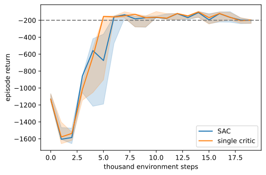
grid = np.arange(1, num_env_steps // 1000 + 1) * 1000

def on_grid(arm, col, k=5):
    """Trailing-k-episode averages, resampled onto the env-step grid."""
    out = []
    for r in runs[arm]:
        v = r[~np.isnan(r[:, col])]
        s = np.convolve(v[:, col], np.ones(k) / k, 'valid')
        out.append(np.interp(grid, v[k - 1:, 0], s))
    return np.stack(out)

def steps_to(r, level=-200, k=5):
    """First env step at which the trailing-k-episode average clears level."""
    s = np.convolve(r[:, 1], np.ones(k) / k, 'valid')
    hit = np.flatnonzero(s >= level)
    return int(r[hit[0] + k - 1, 0]) if len(hit) else None

d2l.plot_curves({arm: on_grid(arm, 1) for arm in runs},
                xlabel='thousand environment steps', ylabel='episode return',
                reference=-200)
for arm in runs:
    print(f'{arm}: env steps to a trailing five-episode average of -200: '
          f'{[steps_to(r) for r in runs[arm]]}')
SAC: env steps to a trailing five-episode average of -200: [7400, 5400, 6400]
single critic: env steps to a trailing five-episode average of -200: [6400, 5400, 7200]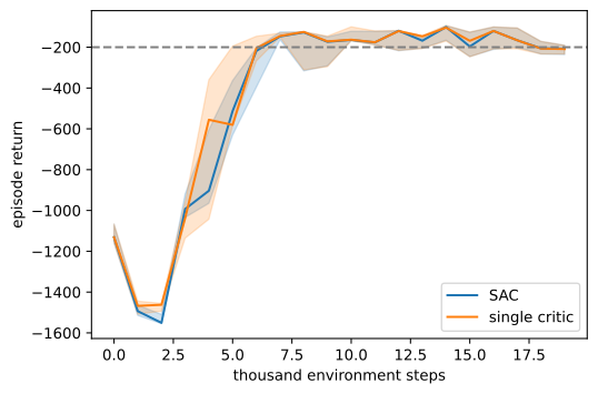
Every seed of both variants starts near \(-1200\) or below and crosses \(-200\) before ten thousand environment steps, most after about five to eight thousand. For comparison, Section 14.7 trained REINFORCE with a learned baseline on the same task for 300 updates of 8 episodes and 200 steps, or \(480{,}000\) environment steps. That experiment reported improvement, but no seed reached \(-200\). The comparison reflects two algorithmic differences. The pathwise gradient differentiates the actor objective through the critic, and replay permits multiple updates from collected transitions. The two variants are not distinguishable in this plot: their uncertainty bands overlap throughout training, and their crossing times have no consistent ordering across frameworks. At this budget, any effect of the second critic is not visible in the return curves, as in the two-action comparison in Section 15.4. The final experiment instead examines critic calibration.
15.5.4.2 Policy Entropy and Temperature
The training loop records policy entropy because its coefficient \(\alpha\) sets the objective’s reward–entropy tradeoff. The dashed line shows the commonly used autotuning target \(-\dim\mathcal{A}=-1\):
d2l.plot_curves({arm: on_grid(arm, 2) for arm in runs},
                xlabel='thousand environment steps',
                ylabel='policy entropy (nats)', reference=-1)
for arm in runs:
    print(f'{arm}: entropy over the last 20 episodes, per seed '
          f'{np.round([np.nanmean(r[-20:, 2]) for r in runs[arm]], 2)}')
SAC: entropy over the last 20 episodes, per seed [-0.03 0.04 0.07]
single critic: entropy over the last 20 episodes, per seed [-0.06 0.12 0.24]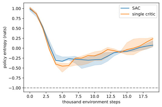
d2l.plot_curves({arm: on_grid(arm, 2) for arm in runs},
                xlabel='thousand environment steps',
                ylabel='policy entropy (nats)', reference=-1)
for arm in runs:
    print(f'{arm}: entropy over the last 20 episodes, per seed '
          f'{np.round([np.nanmean(r[-20:, 2]) for r in runs[arm]], 2)}')
SAC: entropy over the last 20 episodes, per seed [-0.18 0.07 -0.12]
single critic: entropy over the last 20 episodes, per seed [ 0.01 0.15 -0.03]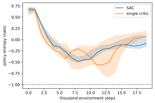
The trace begins high, falls during the period of rapid return improvement, and finishes near zero in both ablations. The policy remains stochastic; for differential entropy, zero has no special status and negative values simply indicate a sufficiently concentrated density.
Reported entropy depends on the density convention. We retain the \(\log c\) term in Equation 15.5.4; an implementation that omits it would report the same policy lower by \(\log 2\approx0.69\) nats in this environment. Entropy values should therefore be compared only after checking the action-scale convention.
We fix \(\alpha=0.2\) in this diagnostic. The resulting entropy happens to finish within about one nat of the common target \(\bar H=-\dim\mathcal{A}=-1\), but this single run does not justify the coefficient generally. Temperature autotuning instead adjusts \(\alpha\) to enforce a chosen entropy constraint (Haarnoja, Zhou, Hartikainen, et al. 2018). The coefficient has units of reward per nat and is reward-scale dependent; it is not a learning rate.
Training returns are generated by the stochastic policy because entropy is part of the objective. We therefore evaluate both that policy and the deterministic mean action \(c\tanh(\mu_\theta(s))\):
env = gym.make('Pendulum-v1')
for arm in runs:
    for seed in range(num_seeds):
        agent = agents[arm][seed]
        env.reset(seed=100 + seed)
        g = d2l.evaluate(env, agent.actor.act_greedy, num_episodes=20)
        env.reset(seed=100 + seed)
        s = d2l.evaluate(env, agent.actor.act, num_episodes=20,
                         rng=np.random.default_rng(1000 + seed))
        print(f'{arm}, seed {seed}: deterministic {g:7.1f}, '
              f'stochastic {s:7.1f}, noise cost {g - s:+6.1f}')
SAC, seed 0: deterministic -184.5, stochastic -184.7, noise cost +0.2
SAC, seed 1: deterministic -141.9, stochastic -148.4, noise cost +6.5
SAC, seed 2: deterministic -184.2, stochastic -184.5, noise cost +0.3
single critic, seed 0: deterministic -183.6, stochastic -182.7, noise cost -0.9
single critic, seed 1: deterministic -146.6, stochastic -147.7, noise cost +1.1
single critic, seed 2: deterministic -183.3, stochastic -183.5, noise cost +0.2env = gym.make('Pendulum-v1')
for arm in runs:
for seed in range(num_seeds):
agent = agents[arm][seed]
env.reset(seed=100 + seed)
g = d2l.evaluate(env, agent.actor.act_greedy, num_episodes=20)
env.reset(seed=100 + seed)
s = d2l.evaluate(env, agent.actor.act, num_episodes=20,
rng=np.random.default_rng(1000 + seed))
print(f'{arm}, seed {seed}: deterministic {g:7.1f}, '
f'stochastic {s:7.1f}, noise cost {g - s:+6.1f}')SAC, seed 0: deterministic -188.8, stochastic -189.8, noise cost +1.0
SAC, seed 1: deterministic -139.0, stochastic -145.8, noise cost +6.9
SAC, seed 2: deterministic -182.5, stochastic -182.5, noise cost -0.0
single critic, seed 0: deterministic -180.8, stochastic -181.2, noise cost +0.5
single critic, seed 1: deterministic -145.1, stochastic -145.9, noise cost +0.8
single critic, seed 2: deterministic -182.1, stochastic -182.1, noise cost +0.0Across variants and frameworks, deterministic returns lie between about \(-140\) and \(-190\), and the stochastic policy is within about ten points of its deterministic counterpart. The learned state-dependent standard deviation therefore preserves entropy with little loss of return on this task. Unlike fixed \(\epsilon\)-greedy exploration, the stochasticity is optimized jointly with the policy under the entropy-regularized objective.
15.5.4.3 Critic Calibration: Predicted and Realized Returns
The critic variants differ more clearly in calibration than in return. For each trained agent, we run twenty stochastic episodes and compare \(\min_j Q_{w_j}(s_0,a_0)\) with the realized return. A soft critic predicts the entropy-regularized return \(\sum_t \gamma^t(r_t-\alpha\log\pi(a_t\mid s_t))\), so this quantity is the appropriate target; the ordinary return is reported alongside it.
def calibration(agent, seed, num_episodes=20):
    """Predicted min_j Q(s0, a0) against the realized discounted soft return."""
    rng, env = np.random.default_rng(seed), gym.make('Pendulum-v1')
    env.reset(seed=seed)
    preds, softs, plains = [], [], []
    for _ in range(num_episodes):
        obs, done, disc = env.reset()[0], False, 1.0
        soft = plain = 0.0
        first = True
        while not done:
            with torch.no_grad():
                mean, std = agent.actor(torch.as_tensor(obs))
                u = mean + std * torch.as_tensor(rng.standard_normal(
                    mean.shape, dtype=np.float32))
                logp = float(agent.actor.log_prob(u, mean, std))
            a = c * np.tanh(u.numpy())
            if first:
                with torch.no_grad():
                    preds.append(float(agent.min_q(
                        torch.as_tensor(obs), torch.as_tensor(a))))
                first = False
            obs, rew, terminated, truncated, _ = env.step(a)
            done = terminated or truncated
            soft += disc * (rew - alpha * logp)
            plain += disc * rew
            disc *= gamma
        softs.append(soft)
        plains.append(plain)
    return np.mean(preds), np.mean(softs), np.mean(plains)

for arm in runs:
    for seed in range(num_seeds):
        pred, soft, plain = calibration(agents[arm][seed], 200 + seed)
        print(f'{arm:>13}, seed {seed}: promised {pred:7.1f}, delivered '
              f'(soft) {soft:7.1f}, gap {pred - soft:+6.1f}, plain {plain:7.1f}')
SAC, seed 0: promised -175.1, delivered (soft) -117.9, gap -57.1, plain -126.4
SAC, seed 1: promised -127.0, delivered (soft) -89.7, gap -37.3, plain -98.1
SAC, seed 2: promised -177.1, delivered (soft) -135.6, gap -41.6, plain -141.9
single critic, seed 0: promised -119.6, delivered (soft) -113.0, gap -6.6, plain -119.3
single critic, seed 1: promised -86.5, delivered (soft) -81.8, gap -4.7, plain -93.7
single critic, seed 2: promised -144.2, delivered (soft) -129.9, gap -14.3, plain -138.3def calibration(agent, seed, num_episodes=20):
"""Predicted min_j Q(s0, a0) against the realized discounted soft return."""
rng, env = np.random.default_rng(seed), gym.make('Pendulum-v1')
env.reset(seed=seed)
preds, softs, plains = [], [], []
for _ in range(num_episodes):
obs, done, disc = env.reset()[0], False, 1.0
soft = plain = 0.0
first = True
while not done:
mean, std = agent.actor(jnp.asarray(obs))
u = np.asarray(mean) + np.asarray(std) * rng.standard_normal(
mean.shape, dtype=np.float32)
logp = float(agent.actor.log_prob(jnp.asarray(u), mean, std))
a = c * np.tanh(u)
if first:
preds.append(float(agent.min_q(jnp.asarray(obs),
jnp.asarray(a))))
first = False
obs, rew, terminated, truncated, _ = env.step(a)
done = terminated or truncated
soft += disc * (rew - alpha * logp)
plain += disc * rew
disc *= gamma
softs.append(soft)
plains.append(plain)
return np.mean(preds), np.mean(softs), np.mean(plains)
for arm in runs:
for seed in range(num_seeds):
pred, soft, plain = calibration(agents[arm][seed], 200 + seed)
print(f'{arm:>13}, seed {seed}: promised {pred:7.1f}, delivered '
f'(soft) {soft:7.1f}, gap {pred - soft:+6.1f}, plain {plain:7.1f}') SAC, seed 0: promised -151.5, delivered (soft) -112.1, gap -39.4, plain -118.1
SAC, seed 1: promised -115.0, delivered (soft) -83.5, gap -31.5, plain -93.3
SAC, seed 2: promised -184.2, delivered (soft) -136.7, gap -47.5, plain -141.3
single critic, seed 0: promised -112.1, delivered (soft) -109.8, gap -2.3, plain -118.8
single critic, seed 1: promised -80.5, delivered (soft) -82.8, gap +2.4, plain -93.1
single critic, seed 2: promised -162.6, delivered (soft) -134.2, gap -28.4, plain -141.8The result is consistent across seeds and frameworks. Neither variant substantially overestimates the realized soft return. The single critic’s prediction is typically within thirty points, whereas the minimum of two critics underestimates the return by about thirty to sixty points. The absolute gap is larger for the twin-critic variant on every seed, consistent with taking a minimum. Some underestimation may also arise because the policy continues to improve while the critic tracks earlier data, so the comparison between variants is more informative than their absolute offsets. On Pendulum, the second critic changes calibration without improving the final policy. On harder tasks, pessimistic targets are intended to reduce feedback between critic overestimation and actor updates; Section 15.6 uses related ideas without further interaction.
15.5.5 Summary
SAC optimizes expected reward plus entropy. Soft policy evaluation adds \(-\alpha\log\pi\) to the bootstrap target, and soft policy improvement uses a pathwise gradient through the critic. A tanh transformation enforces bounded actions; its log density must include the change-of-variables determinant, evaluated in a numerically stable form. Replay, Polyak-averaged target networks, and the minimum of two critics provide the off-policy value-learning machinery. No target actor or importance ratios are required.
Experimental scope. The density and soft-backup checks are deterministic. Training uses three seeds per method and framework. Every SAC run reaches return \(-200\) within \(10{,}000\) environment steps on Pendulum, while deterministic final evaluations lie roughly between \(-140\) and \(-190\). Twin and single critics have similar returns at this budget; the twin-critic minimum is more pessimistic in every calibration comparison. Exact crossing times and calibration gaps vary across seeds.
15.5.6 Exercises
- [short-code] Autotune the temperature. (Haarnoja, Zhou, Hartikainen, et al. 2018) replaces the fixed \(\alpha\) by a constraint \(E\big[ H(\pi(\cdot \mid s_t)) \big] \geq \bar{H}\) with \(\bar{H} = -\dim \mathcal{A}\), and lets \(\alpha\) be the Lagrange multiplier, minimizing \(J(\alpha) = E_{a \sim \pi}\big[ -\alpha (\log \pi(a \mid s) + \bar{H}) \big]\) by gradient steps on \(\log \alpha\). Add this to
train_sac(a few lines: one extra parameter, updated from thelogpthe loop already computes), starting from \(\alpha_0 = 1\). Plot \(\alpha_t\) and the entropy trace. Does the entropy converge to \(\bar{H}\), and where does \(\alpha\) end up relative to the \(0.2\) we fixed? - [short-code] Delete the log-determinant. Remove the
logdetterm fromlog_proband retrain one seed. Report three readings: the return curve, the entropy trace, and the quadrature check. Which diagnostics expose the error, and why can the return curve fail to do so? - [conceptual] Off-policy without ratios. For each expectation in Equation 15.5.2 and Equation 15.5.3, state the distribution it is taken under and which part the replay buffer supplies. Where Section 15.2 needed importance ratios, why does nothing here need one, and what distribution shift does the buffer still introduce that no ratio over actions can repair?
- [short-code] Entropy is not monotone in the noise. Estimate the squashed policy’s entropy \(-E[\log \pi]\) at fixed \(\mu = 0\) and \(\sigma \in \{0.1, 0.3, 1, 3\}\) by sampling \(u\) and averaging
log_prob(do not integrate over the action: the density near the boundary defeats a uniform grid). Explain why the entropy peaks at an intermediate \(\sigma\) and falls as mass piles onto the boundary, and what that implies for an agent trying to raise its entropy by inflating \(\sigma\). - [short-code] The limit \(\alpha \to 0\) is DDPG. Show numerically that at \(\alpha = 0\) and \(\sigma \to 0\) the actor’s gradient in Equation 15.5.3 equals the pathwise gradient of Equation 14.7.1 evaluated at the deterministic action \(c \tanh(\mu_\theta(s))\), which is DDPG’s actor update (Lillicrap et al. 2016). Then list TD3’s three repairs (Fujimoto et al. 2018) and say which two SAC kept and why the stochastic policy makes the third unnecessary.
- [short-code] Port it. Move the section’s code to
LunarLander-v3withcontinuous=True, whose action is two-dimensional. List every line that changes and every line that does not, in the spirit of Section 15.4’s port exercise; say which single hyperparameter you expect to raise most and why; check thatlog_probstill reduces correctly over the action axis; and explain what breaks, and where, if you instead port toCartPole-v1. - [extended] Discrete soft actor-critic. With a finite action set both expectations in Equation 15.5.2 and Equation 15.5.3 can be computed exactly by summing over actions, and no reparameterization is needed. Write both losses for a softmax policy, state what replaces the tanh machinery, and implement it on CartPole; compare its sample efficiency against Section 15.4’s DQN at the same step budget.