from d2l import torch as d2l
import numpy as np
import torch
from torch import nn2.5 Concise Implementation of Linear Regression
In Section 2.4 we initialized the parameters, defined the forward pass and squared loss, and implemented the update explicitly. Modern frameworks provide reusable implementations of each of these components. This section rebuilds the same model with framework data loaders, layers, losses, and optimizers, identifying the primitive that replaces each explicit step.
from d2l import tensorflow as d2l
import numpy as np
import tensorflow as tf
from d2l import jax as d2l
from flax import nnx
import jax
from jax import numpy as jnp
import optaxfrom d2l import mxnet as d2l
from mxnet import autograd, gluon, init, np, npx
from mxnet.gluon import nn
npx.set_np()2.5.1 Defining the Model
Each component from Section 2.4 has a direct counterpart here. The hand-rolled weight vector \(\mathbf{w}\) and bias \(b\) are replaced by a single layer; our manual squared-error computation is replaced by a built-in loss; and our explicit parameter-update loop is replaced by an optimizer object. Implementing these components once exposes their behavior. For routine work, framework components reduce repeated code and provide optimized implementations.
For standard operations, we can use a framework’s predefined layers, which allow us to focus on the layers used to construct the model rather than worrying about their implementation. Recall the architecture of a single-layer network as described in Figure 2.1.3. The layer is called fully connected, since each of its inputs is connected to each of its outputs by means of a matrix–vector multiplication.
In PyTorch, the fully connected layer is defined in Linear and LazyLinear classes (available since version 1.8.0). The latter requires only the output dimension, while the former additionally asks for how many inputs go into this layer. Specifying input shapes is inconvenient and may require nontrivial calculations (such as in convolutional layers). Thus, for simplicity, we will use such “lazy” layers whenever we can.
In Keras, the fully connected layer is defined in the Dense class. Since we only want to generate a single scalar output, we set that number to 1. For convenience, Keras does not require us to specify the input shape for each layer. We do not need to tell Keras how many inputs go into this linear layer. When we first try to pass data through our model, e.g., when we execute net(X) later, Keras will automatically infer the number of inputs to each layer. We will describe how this works in more detail later.
In Gluon, the fully connected layer is defined in the Dense class. Since we only want to generate a single scalar output, we set that number to 1. For convenience, Gluon does not require us to specify the input shape for each layer. Hence we do not need to tell Gluon how many inputs go into this linear layer. When we first pass data through our model, e.g., when we execute net(X) later, Gluon will automatically infer the number of inputs to each layer and thus instantiate the correct model. We will describe how this works in more detail later.
class LinearRegression(d2l.Module):
    """The linear regression model implemented with high-level APIs."""
    def __init__(self, lr):
        super().__init__()
        self.save_hyperparameters()
        self.net = nn.LazyLinear(1)
class LinearRegression(d2l.Module):
"""The linear regression model implemented with high-level APIs."""
def __init__(self, lr):
super().__init__()
self.save_hyperparameters()
initializer = tf.initializers.RandomNormal(stddev=0.01)
self.net = tf.keras.layers.Dense(1, kernel_initializer=initializer)class LinearRegression(d2l.Module):
"""The linear regression model implemented with high-level APIs."""
def __init__(self, num_inputs, lr, rngs=None):
super().__init__()
self.save_hyperparameters(ignore=['rngs'])
rngs = nnx.Rngs(d2l.get_key()) if rngs is None else rngs
self.net = nnx.Linear(
num_inputs, 1, kernel_init=nnx.initializers.normal(0.01),
rngs=rngs)class LinearRegression(d2l.Module):
"""The linear regression model implemented with high-level APIs."""
def __init__(self, lr):
super().__init__()
self.save_hyperparameters()
self.net = nn.Dense(1)
self.net.initialize(init.Normal(sigma=0.01))The forward method invokes the predefined layer’s built-in __call__ method.
@d2l.add_to_class(LinearRegression)
def forward(self, X):
return self.net(X)@d2l.add_to_class(LinearRegression)
def forward(self, X):
return self.net(X)@d2l.add_to_class(LinearRegression)
def forward(self, X):
return self.net(X)@d2l.add_to_class(LinearRegression)
def forward(self, X):
return self.net(X)2.5.2 Defining the Loss Function
The MSELoss class computes the mean squared error (without the \(1/2\) factor in Equation 2.1.4). By default, MSELoss returns the average loss over examples. Using the library primitive also gives us its tested reduction and automatic-differentiation behavior; performance should be measured rather than assumed.
The MeanSquaredError class computes the mean squared error (without the \(1/2\) factor in Equation 2.1.4). By default, it returns the average loss over examples.
The loss module defines many useful loss functions. We choose the built-in loss.L2Loss rather than maintaining another implementation. Because the loss that it returns is the squared error for each example, we use mean to average the loss over the minibatch.
@d2l.add_to_class(LinearRegression)
def loss(self, y_hat, y):
    fn = nn.MSELoss()
return fn(y_hat, y)@d2l.add_to_class(LinearRegression)
def loss(self, y_hat, y):
fn = tf.keras.losses.MeanSquaredError()
return fn(y, y_hat)@d2l.add_to_class(LinearRegression)
def loss(self, y_hat, y):
return d2l.reduce_mean(jnp.square(y_hat - y))@d2l.add_to_class(LinearRegression)
def loss(self, y_hat, y):
fn = gluon.loss.L2Loss()
return 2 * fn(y_hat, y).mean() # Gluon's L2Loss includes 1/2; multiply by 2 to get plain MSE2.5.3 Defining the Optimization Algorithm
Minibatch SGD is a standard tool for optimizing neural networks and thus PyTorch supports it alongside a number of variations on this algorithm in the optim module. When we instantiate an SGD instance, we specify the parameters to optimize over, obtainable from our model via self.parameters(), and the learning rate (self.lr) required by our optimization algorithm.
Minibatch SGD is a standard tool for optimizing neural networks and thus Keras supports it alongside a number of variations on this algorithm in the optimizers module.
Minibatch SGD is a standard tool for optimizing neural networks and thus Gluon supports it alongside a number of variations on this algorithm through its Trainer class. Note that Gluon’s Trainer class stands for the optimization algorithm, while the Trainer class we created in Section 2.2 contains the training method, i.e., repeatedly call the optimizer to update the model parameters. When we instantiate Trainer, we specify the parameters to optimize over, obtainable from our model net via net.collect_params(), the optimization algorithm we wish to use (sgd), and a dictionary of hyperparameters required by our optimization algorithm.
@d2l.add_to_class(LinearRegression)
def configure_optimizers(self):
return torch.optim.SGD(self.parameters(), self.lr)@d2l.add_to_class(LinearRegression)
def configure_optimizers(self):
return tf.keras.optimizers.SGD(self.lr)@d2l.add_to_class(LinearRegression)
def configure_optimizers(self):
return optax.sgd(self.lr)@d2l.add_to_class(LinearRegression)
def configure_optimizers(self):
return gluon.Trainer(self.collect_params(),
'sgd', {'learning_rate': self.lr})2.5.4 Training
Expressing the model through high-level framework APIs requires fewer lines of code. We did not have to allocate parameters individually, define our loss function, or implement minibatch SGD. Once we start working with much more complex models, the advantages of the high-level API will grow considerably.
The batch-level computation is now delegated to standard layers, loss, and optimizer objects, while the training loop is the same one used from scratch. We call the fit method (introduced in Section 2.2.4), which relies on the implementation of the fit_epoch method in Section 2.4, to train our model.
model = LinearRegression(lr=0.03)
data = d2l.SyntheticRegressionData(w=d2l.tensor([2, -3.4]), b=4.2)
# Materialize lazy parameters before replacing their default initialization.
model(data.X[:1])
with torch.no_grad():
    model.net.weight.normal_(0, 0.01)
    model.net.bias.fill_(0)
trainer = d2l.Trainer(max_epochs=10)
trainer.fit(model, data)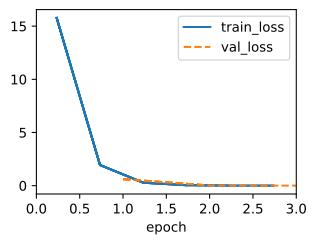
model = LinearRegression(lr=0.03)
data = d2l.SyntheticRegressionData(w=d2l.tensor([2, -3.4]), b=4.2)
trainer = d2l.Trainer(max_epochs=10)
trainer.fit(model, data)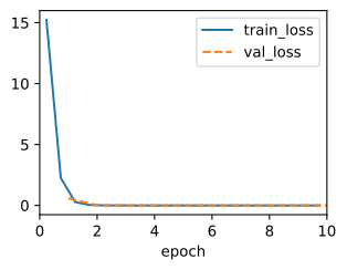
model = LinearRegression(2, lr=0.03)
data = d2l.SyntheticRegressionData(w=d2l.tensor([2, -3.4]), b=4.2)
trainer = d2l.Trainer(max_epochs=10)
trainer.fit(model, data)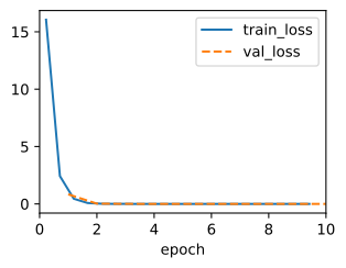
model = LinearRegression(lr=0.03)
data = d2l.SyntheticRegressionData(w=d2l.tensor([2, -3.4]), b=4.2)
trainer = d2l.Trainer(max_epochs=10)
trainer.fit(model, data)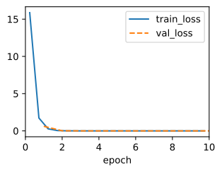
Below, we compare the model parameters learned by training on finite data and the actual parameters that generated our dataset. This is where the concise version differs conceptually from the scratch one: the parameters no longer hang off our class as self.w and self.b but live inside the layer object, so get_w_b reaches through net to find them. As in our implementation from scratch, note that our estimated parameters are close to their true counterparts.
@d2l.add_to_class(LinearRegression)
def get_w_b(self):
    return (self.net.weight.detach(), self.net.bias.detach())
w, b = model.get_w_b()@d2l.add_to_class(LinearRegression)
def get_w_b(self):
return (self.get_weights()[0], self.get_weights()[1])
w, b = model.get_w_b()@d2l.add_to_class(LinearRegression)
def get_w_b(self):
return self.net.kernel[...], self.net.bias[...]
w, b = model.get_w_b()@d2l.add_to_class(LinearRegression)
def get_w_b(self):
return (self.net.weight.data(), self.net.bias.data())
w, b = model.get_w_b()print(f'error in estimating w: {data.w - d2l.reshape(w, data.w.shape)}')
print(f'error in estimating b: {data.b - b}')error in estimating w: tensor([ 4.7922e-05, -2.0504e-04])
error in estimating b: tensor([-0.0002])error in estimating w: [6.532669e-05 7.343292e-05]
error in estimating b: [2.336502e-05]error in estimating w: [-2.6226044e-05 -1.8382072e-04]
error in estimating b: [0.00037479]error in estimating w: [-4.6229362e-04 4.4822693e-05]
error in estimating b: [0.00054073]2.5.5 Summary
MXNet (Chen et al. 2015), JAX (Frostig et al. 2018), PyTorch (Paszke et al. 2019), and TensorFlow (Abadi et al. 2016) provide standard implementations of data loaders, layers, losses, optimizers, and training utilities. These components are concise, tested, and optimized. Direct implementations remain useful when a model requires a component that the framework does not provide.
In PyTorch, the data module provides tools for data processing, the nn module defines a large number of neural network layers and common loss functions. Because we used nn.LazyLinear, the input dimensions are inferred automatically on the first forward pass. Before that pass, the layer contains UninitializedParameter placeholders: writing to them does not initialize the eventual weights. The training cell therefore makes a one-example dry run and then initializes the materialized parameters inside torch.no_grad(). This lazy shape inference pays off in deeper networks (convolutional layers, variable-length sequences), where computing the input size of each layer by hand would be tedious and error-prone.
In TensorFlow, the data module provides tools for data processing, the keras module defines a large number of neural network layers and common loss functions. Moreover, the initializers module provides various methods for model parameter initialization. Dimensionality and storage for networks are automatically inferred (but be careful not to attempt to access parameters before they have been initialized).
In Gluon, the data module provides tools for data processing, the nn module defines a large number of neural network layers, and the loss module defines many common loss functions. Moreover, the initializer gives access to many choices for parameter initialization. Conveniently for the user, dimensionality and storage are automatically inferred. A consequence of this lazy initialization is that you must not attempt to access parameters before they have been instantiated (and initialized).
2.5.6 Exercises
Sum versus mean. The framework loss functions used above return the mean loss over the minibatch by default. State how the learning rate must change if you replace this average with the sum of the losses over the minibatch, e.g., by passing
reduction='sum', and explain why.[code] Huber loss. Review the framework documentation to see which loss functions are provided. In particular, replace the squared loss with Huber’s robust loss function
\[l(y,y') = \begin{cases}|y-y'| -\frac{\sigma}{2} & \textrm{ if } |y-y'| > \sigma \\ \frac{1}{2 \sigma} (y-y')^2 & \textrm{ otherwise.}\end{cases} \tag{2.5.1}\]
Rerun the outlier demonstration of Section 2.1.1.2 with one corrupted label. Report whether Huber’s loss recovers the robust estimate, the least-squares one, or something in between, and relate the outcome to the penalty curves in Figure 2.1.2.
[code] Reading gradients. Show how to access the gradient of the model’s weights after one backward pass, and confirm that it matches the by-hand gradient formula from Section 2.4.
[code] Learning-rate and epoch grid. Train the concise model at each combination of learning rate in \(\{0.01, 0.03, 0.1, 0.3\}\) and epoch count in \(\{5, 10, 30\}\). Report the final loss for all twelve combinations in a small table, and state which combinations fail to improve on the default configuration.
[code] Sample-size scaling. How does the solution change as you vary the amount of data generated?
- Plot the estimation error for \(\hat{\mathbf{w}} - \mathbf{w}\) and \(\hat{b} - b\) as a function of the amount of data. Hint: increase the amount of data logarithmically rather than linearly, i.e., 5, 10, 20, 50, …, 10,000 rather than 1000, 2000, …, 10,000.
- Explain why the suggestion in the hint is appropriate.
[code] Scratch versus concise. Time the from-scratch implementation of Section 2.4 against the concise one here, training each for 10, 100, and 1,000 epochs on the same synthetic dataset. Report which is faster and whether the gap grows with the number of epochs, and state what this shows about the overhead of Python-level parameter bookkeeping versus framework-optimized operations.