22.3 Asynchronous Random Search

As we have seen in the previous Section 22.2, we might have to wait hours or even days before random search returns a good hyperparameter configuration, because of the expensive evaluation of hyperparameter configurations. In practice, we have often access to a pool of resources such as multiple GPUs on the same machine or multiple machines with a single GPU. This begs the question: How do we efficiently distribute random search?

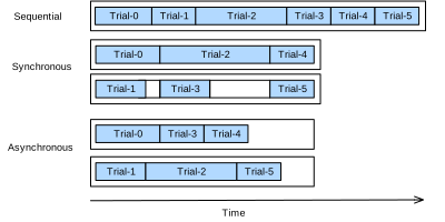
In general, we distinguish between synchronous and asynchronous parallel hyperparameter optimization (see Figure 22.3.1). In the synchronous setting, we wait for all concurrently running trials to finish, before we start the next batch. Consider configuration spaces that contain hyperparameters such as the number of filters or number of layers of a deep neural network. Hyperparameter configurations that contain a larger number of layers of filters will naturally take more time to finish, and all other trials in the same batch will have to wait at synchronization points (grey area in Figure 22.3.1) before we can continue the optimization process.

In the asynchronous setting we immediately schedule a new trial as soon as resources become available. This will optimally exploit our resources, since we can avoid any synchronization overhead. For random search, each new hyperparameter configuration is chosen independently of all others, and in particular without exploiting observations from any prior evaluation. This means we can trivially parallelize random search asynchronously. This is not straightforward with more sophisticated methods that make decision based on previous observations (see Section 22.5). While we need access to more resources than in the sequential setting, asynchronous random search exhibits a linear speed-up, in that a certain performance is reached \(K\) times faster if \(K\) trials can be run in parallel.

Figure 22.3.1: Distributing the hyperparameter optimization process either synchronously or asynchronously. Compared to the sequential setting, we can reduce the overall wall-clock time while keep the total compute constant. Synchronous scheduling might lead to idling workers in the case of stragglers.

In this section, we will look at asynchronous random search where trials are executed in multiple python processes on the same machine. Distributed job scheduling and execution is difficult to implement from scratch. We will use Syne Tune (Salinas et al. 2022), which provides us with a simple interface for asynchronous HPO. Syne Tune is designed to be run with different execution back-ends, and the interested reader is invited to study its simple APIs in order to learn more about distributed HPO.

from d2l import torch as d2l
import logging
# Use INFO level so the periodic Syne Tune tuning-status table appears,
# but use a clean format that drops the "INFO:syne_tune.tuner:" prefix.
logging.basicConfig(level=logging.INFO, format="%(message)s", force=True)
# Silence Syne Tune's import-time chatter about optional AWS dependencies
# (sagemaker, s3fs) and Ray Tune. We use the local PythonBackend, so those
# are not needed. Suppress both print() and logging.info() during imports.
import contextlib, io
_root = logging.getLogger()
_prev_level = _root.level
_root.setLevel(logging.WARNING)
try:
    with contextlib.redirect_stdout(io.StringIO()):
        from syne_tune.config_space import loguniform, randint
        from syne_tune.backend.python_backend.python_backend import PythonBackend
        from syne_tune.optimizer.baselines import RandomSearch
        from syne_tune import Tuner, StoppingCriterion
        from syne_tune.experiments import load_experiment
finally:
    _root.setLevel(_prev_level)

# Silence the per-trial subprocess-command spam from local_backend and
# drop the per-trial scheduling / completion lines from the tuner logger.
# Keep the periodic "tuning status (last metric is reported)" updates so
# the reader can still see progress over time.
class _DropPerTrialNoise(logging.Filter):
    _DROP = (
        "results of trials will be saved",
        "scheduled ",
        "Trial trial_id ",
    )
    def filter(self, record):
        msg = record.getMessage()
        return not any(s in msg for s in self._DROP)

logging.getLogger("syne_tune.backend.local_backend").setLevel(logging.WARNING)
logging.getLogger("syne_tune.tuner").addFilter(_DropPerTrialNoise())

22.3.1 Objective Function

First, we have to define a new objective function such that it now returns the performance back to Syne Tune via the report callback.

def hpo_objective_lenet_synetune(learning_rate, batch_size, max_epochs):
    from d2l import torch as d2l    
    from syne_tune import Reporter

    model = d2l.LeNet(lr=learning_rate, num_classes=10)
    trainer = d2l.HPOTrainer(max_epochs=1, num_gpus=1)
    data = d2l.FashionMNIST(batch_size=batch_size)
    model.apply_init([next(iter(data.get_dataloader(True)))[0]], d2l.init_cnn)
    report = Reporter() 
    for epoch in range(1, max_epochs + 1):
        if epoch == 1:
            # Initialize the state of Trainer
            trainer.fit(model=model, data=data) 
        else:
            trainer.fit_epoch()
        validation_error = d2l.numpy(trainer.validation_error().cpu())
        report(epoch=epoch, validation_error=float(validation_error))

Note that the PythonBackend of Syne Tune requires dependencies to be imported inside the function definition.

22.3.2 Asynchronous Scheduler

First, we define the number of workers that evaluate trials concurrently. We also need to specify how long we want to run random search, by defining an upper limit on the total wall-clock time.

# Each LeNet trial fits in well under 7 GB of GPU memory, so we can pack
# multiple trials per device. `PythonBackend(rotate_gpus=True)` (the
# default) round-robins trials across detected GPUs and falls back to
# sharing when `n_workers > num_gpus`. Allocate 7 GB per slot — this
# yields 3 slots on a 24 GB card and 4 slots on a 32 GB card after
# driver overhead, e.g. 4×24 GB → 12 slots; 2×32 GB → 8.
import torch
_GB = 1024 ** 3
n_workers = sum(
    torch.cuda.get_device_properties(i).total_memory // (7 * _GB)
    for i in range(torch.cuda.device_count())
) or 1

max_wallclock_time = 15 * 60  # 15 minutes

Next, we state which metric we want to optimize and whether we want to minimize or maximize this metric. Namely, metric needs to correspond to the argument name passed to the report callback.

mode = "min"
metric = "validation_error"

We use the configuration space from our previous example. In Syne Tune, this dictionary can also be used to pass constant attributes to the training script. We make use of this feature in order to pass max_epochs. Moreover, we specify the first configuration to be evaluated in initial_config.

config_space = {
    "learning_rate": loguniform(1e-2, 1),
    "batch_size": randint(32, 256),
    "max_epochs": 10,
}
initial_config = {
    "learning_rate": 0.1,
    "batch_size": 128,
}

Next, we need to specify the back-end for job executions. Here we just consider the distribution on a local machine where parallel jobs are executed as sub-processes. However, for large scale HPO, we could run this also on a cluster or cloud environment, where each trial consumes a full instance.

trial_backend = PythonBackend(
    tune_function=hpo_objective_lenet_synetune,
    config_space=config_space,
)

We can now create the scheduler for asynchronous random search, which is similar in behaviour to our BasicScheduler from Section 22.2.

scheduler = RandomSearch(
    config_space,
    metric=metric,
    mode=mode,
    points_to_evaluate=[initial_config],
)

max_resource_level = 10, as inferred from config_space
Master random_seed = 33997532

Syne Tune also features a Tuner, where the main experiment loop and bookkeeping is centralized, and interactions between scheduler and back-end are mediated.

stop_criterion = StoppingCriterion(max_wallclock_time=max_wallclock_time)

tuner = Tuner(
    trial_backend=trial_backend,
    scheduler=scheduler, 
    stop_criterion=stop_criterion,
    n_workers=n_workers,
    print_update_interval=int(max_wallclock_time * 0.6),
)

Let us run our distributed HPO experiment. According to our stopping criterion, it will run for about 15 minutes.

tuner.run()

tuning status (last metric is reported)
 trial_id     status  iter  learning_rate  batch_size  max_epochs  epoch  validation_error  worker-time
        0  Completed    10       0.100000         128          10     10          0.270075    39.655056
        1  Completed    10       0.014202         154          10     10          0.899982    37.824496
        2  Completed    10       0.026376         178          10     10          0.900989    36.683783
        3  Completed    10       0.344002         133          10     10          0.240035    37.504084
        4  Completed    10       0.465107         174          10     10          0.191509    34.643521
        5  Completed    10       0.012816          82          10     10          0.873020    45.108681
        6  Completed    10       0.240766         245          10     10          0.262444    31.379914
        7  Completed    10       0.057977          72          10     10          0.272307    47.630770
        8  Completed    10       0.051127         159          10     10          0.407749    33.478391
        9  Completed    10       0.074367         221          10     10          0.422127    31.692682
       10  Completed    10       0.022302         100          10     10          0.900000    39.773550
       11  Completed    10       0.192134          41          10     10          0.155115    71.720723
       12  Completed    10       0.407880         218          10     10          0.249077    31.618427
       13  Completed    10       0.085853          46          10     10          0.213115    64.586580
       14  Completed    10       0.576145         119          10     10          0.176965    36.598821
       15  Completed    10       0.059979         152          10     10          0.372036    33.493336
       16  Completed    10       0.024327         200          10     10          0.900000    31.048553
       17  Completed    10       0.324870         221          10     10          0.239844    30.485928
       18  Completed    10       0.075878         104          10     10          0.271461    38.261357
       19  Completed    10       0.482672          52          10     10          0.142512    58.050390
       20  Completed    10       0.478743         172          10     10          0.178820    32.917817
       21  Completed    10       0.104099         185          10     10          0.309681    32.226314
       22  Completed    10       0.053336          32          10     10          0.219649    90.555779
       23  Completed    10       0.087115         238          10     10          0.457495    30.356888
       24  Completed    10       0.220552         191          10     10          0.264521    31.286900
       25  Completed    10       0.121485         198          10     10          0.424858    31.454133
       26  Completed    10       0.020927          48          10     10          0.336922    67.902298
       27  Completed    10       0.022402         193          10     10          0.899970    30.784399
       28  Completed    10       0.469205         215          10     10          0.249278    30.935999
       29  Completed    10       0.043159         102          10     10          0.370568    38.216198
       30  Completed    10       0.013077         163          10     10          0.900497    32.123291
       31  Completed    10       0.180472         133          10     10          0.245378    34.026652
       32 InProgress     5       0.753940         239          10      5          0.280523    15.299766
       33 InProgress     3       0.769978         218          10      3          0.307194     9.536001
       34 InProgress     1       0.360761         231          10      1          0.900169     3.661032
3 trials running, 32 finished (32 until the end), 541.85s wallclock-time

reaching max wallclock time (900), stopping there.
Stopping trials that may still be running.
Tuning finished, results of trials can be found on syne-tune/python-entrypoint-2026-07-28-18-03-03-364

--------------------
Resource summary (last result is reported):
 trial_id     status  iter  learning_rate  batch_size  max_epochs  epoch  validation_error  worker-time
        0  Completed    10       0.100000         128          10     10          0.270075    39.655056
        1  Completed    10       0.014202         154          10     10          0.899982    37.824496
        2  Completed    10       0.026376         178          10     10          0.900989    36.683783
        3  Completed    10       0.344002         133          10     10          0.240035    37.504084
        4  Completed    10       0.465107         174          10     10          0.191509    34.643521
        5  Completed    10       0.012816          82          10     10          0.873020    45.108681
        6  Completed    10       0.240766         245          10     10          0.262444    31.379914
        7  Completed    10       0.057977          72          10     10          0.272307    47.630770
        8  Completed    10       0.051127         159          10     10          0.407749    33.478391
        9  Completed    10       0.074367         221          10     10          0.422127    31.692682
       10  Completed    10       0.022302         100          10     10          0.900000    39.773550
       11  Completed    10       0.192134          41          10     10          0.155115    71.720723
       12  Completed    10       0.407880         218          10     10          0.249077    31.618427
       13  Completed    10       0.085853          46          10     10          0.213115    64.586580
       14  Completed    10       0.576145         119          10     10          0.176965    36.598821
       15  Completed    10       0.059979         152          10     10          0.372036    33.493336
       16  Completed    10       0.024327         200          10     10          0.900000    31.048553
       17  Completed    10       0.324870         221          10     10          0.239844    30.485928
       18  Completed    10       0.075878         104          10     10          0.271461    38.261357
       19  Completed    10       0.482672          52          10     10          0.142512    58.050390
       20  Completed    10       0.478743         172          10     10          0.178820    32.917817
       21  Completed    10       0.104099         185          10     10          0.309681    32.226314
       22  Completed    10       0.053336          32          10     10          0.219649    90.555779
       23  Completed    10       0.087115         238          10     10          0.457495    30.356888
       24  Completed    10       0.220552         191          10     10          0.264521    31.286900
       25  Completed    10       0.121485         198          10     10          0.424858    31.454133
       26  Completed    10       0.020927          48          10     10          0.336922    67.902298
       27  Completed    10       0.022402         193          10     10          0.899970    30.784399
       28  Completed    10       0.469205         215          10     10          0.249278    30.935999
       29  Completed    10       0.043159         102          10     10          0.370568    38.216198
       30  Completed    10       0.013077         163          10     10          0.900497    32.123291
       31  Completed    10       0.180472         133          10     10          0.245378    34.026652
       32  Completed    10       0.753940         239          10     10          0.335896    30.501931
       33  Completed    10       0.769978         218          10     10          0.197718    31.079966
       34  Completed    10       0.360761         231          10     10          0.235696    30.048576
       35  Completed    10       0.049439          92          10     10          0.361588    40.826263
       36  Completed    10       0.032234          99          10     10          0.490592    39.512521
       37  Completed    10       0.048337         211          10     10          0.900350    31.680078
       38  Completed    10       0.047880         118          10     10          0.436982    37.188029
       39  Completed    10       0.017669         198          10     10          0.900194    32.099723
       40  Completed    10       0.704379         252          10     10          0.302413    30.796555
       41  Completed    10       0.078289          97          10     10          0.262765    39.973924
       42  Completed    10       0.052447          85          10     10          0.294335    42.689931
       43  Completed    10       0.052762         154          10     10          0.441489    33.420151
       44  Completed    10       0.755569         129          10     10          0.162481    34.889941
       45  Completed    10       0.072468         218          10     10          0.404417    31.226071
       46  Completed    10       0.169204         205          10     10          0.293657    31.356803
       47  Completed    10       0.128291          89          10     10          0.235825    41.640538
       48  Completed    10       0.024714          86          10     10          0.442564    43.494969
       49  Completed    10       0.019112          89          10     10          0.671634    43.759704
       50  Completed    10       0.317743         162          10     10          0.225366    33.339402
       51  Completed    10       0.364101         120          10     10          0.174206    37.735651
       52  Completed    10       0.963011         176          10     10          0.167021    32.770046
       53 InProgress     8       0.783203          38          10      8          0.136863    61.063006
       54  Completed    10       0.144396         120          10     10          0.259226    36.739446
       55  Completed    10       0.335394         238          10     10          0.322210    30.858170
       56 InProgress     5       0.015470         103          10      5          0.898862    19.719671
       57 InProgress     6       0.019738         150          10      6          0.836866    20.160092
3 trials running, 55 finished (55 until the end), 904.00s wallclock-time

validation_error: best 0.1368626356124878 for trial-id 53
--------------------

The logs of all evaluated hyperparameter configurations are stored for further analysis. At any time during the tuning job, we can easily get the results obtained so far and plot the incumbent trajectory.

d2l.set_figsize()
tuning_experiment = load_experiment(tuner.name)
tuning_experiment.plot()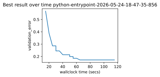

22.3.3 Visualize the Asynchronous Optimization Process

Below we visualize how the learning curves of every trial (each color in the plot represents a trial) evolve during the asynchronous optimization process. At any point in time, there are as many trials running concurrently as we have workers. Once a trial finishes, we immediately start the next trial, without waiting for the other trials to finish. Idle time of workers is reduced to a minimum with asynchronous scheduling.

d2l.set_figsize([6, 2.5])
results = tuning_experiment.results

for trial_id in results.trial_id.unique():
    df = results[results["trial_id"] == trial_id]
    d2l.plt.plot(
        df["st_tuner_time"],
        df["validation_error"],
        marker="o"
    )
    
d2l.plt.xlabel("wall-clock time")
d2l.plt.ylabel("objective function")

Text(0, 0.5, 'objective function')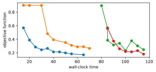

22.3.4 Summary

We can reduce the waiting time for random search substantially by distributing trials across parallel resources. In general, we distinguish between synchronous scheduling and asynchronous scheduling. Synchronous scheduling means that we sample a new batch of hyperparameter configurations once the previous batch finished. If we have stragglers - trials that take more time to finish than other trials - our workers need to wait at synchronization points. Asynchronous scheduling evaluates new hyperparameter configurations as soon as resources become available, and, hence, ensures that all workers are busy at any point in time. While random search is easy to distribute asynchronously and does not require any change of the actual algorithm, other methods require some additional modifications.

22.3.5 Exercises

Consider the DropoutMLP model implemented in Section 4.6, and used in Exercise 1 of Section 22.2.
1. Implement an objective function hpo_objective_dropoutmlp_synetune to be used with Syne Tune. Make sure that your function reports the validation error after every epoch.
2. Using the setup of Exercise 1 in Section 22.2, compare random search to Bayesian optimization. If you use SageMaker, feel free to use Syne Tune’s benchmarking facilities in order to run experiments in parallel. Hint: Bayesian optimization is provided as syne_tune.optimizer.baselines.BayesianOptimization.
3. For this exercise, you need to run on an instance with at least 4 CPU cores. For one of the methods used above (random search, Bayesian optimization), run experiments with n_workers=1, n_workers=2, n_workers=4, and compare results (incumbent trajectories). At least for random search, you should observe linear scaling with respect to the number of workers. Hint: For robust results, you may have to average over several repetitions each.
Advanced. The goal of this exercise is to implement a new scheduler in Syne Tune.
1. Create a virtual environment containing both the d2lbook and syne-tune sources.
2. Implement the LocalSearcher from Exercise 2 in Section 22.2 as a new searcher in Syne Tune. Hint: Read this tutorial. Alternatively, you may follow this example.
3. Compare your new LocalSearcher with RandomSearch on the DropoutMLP benchmark.

PyTorch

Discussions