%matplotlib inline
from d2l import torch as d2l
import numpy as np27.4 Bayesian Computation
Maximum-likelihood and MAP estimation each return a single parameter vector. When the data leave substantial parameter uncertainty, different plausible vectors can produce different predictions. Bayesian prediction averages these predictions with respect to the posterior distribution. The resulting posterior predictive distribution is
\[ p(y_\star\mid\mathbf x_\star,\mathcal D) =\int p(y_\star\mid\mathbf x_\star,\boldsymbol\theta)\, p(\boldsymbol\theta\mid\mathcal D)\,d\boldsymbol\theta. \tag{27.4.1}\]
Outside the conjugate families of Section 27.2, this integral — and the posterior’s own normalizer — usually has no closed form. We can evaluate the unnormalized posterior pointwise, but must approximate its integrals. This leads to the computational question:
How do you average over a distribution you can only evaluate pointwise, up to a constant?
This section develops four approximations. Importance sampling draws from a tractable proposal and reweights the samples. Markov chain Monte Carlo constructs a chain whose stationary distribution is the posterior. The Laplace approximation fits a Gaussian near a posterior mode. Variational inference optimizes a tractable distribution to approximate the posterior. These methods are used for posterior prediction, uncertainty estimates, and latent-variable models.
One Bayesian logistic-regression problem provides a common comparison. Because it has only two parameters, a sufficiently fine grid supplies a high-accuracy numerical reference for checking the approximations. Conjugate posteriors are treated in Section 27.2; MAP and the ELBO are developed in Section 27.3; differentiation through random variables is in Section 25.4.5.1.1. Standard broader references are Bishop (2006) and Murphy (2022) . All computation is plain NumPy.
%matplotlib inline
from d2l import tensorflow as d2l
import numpy as np%matplotlib inline
from d2l import jax as d2l
import numpy as np%matplotlib inline
from d2l import mxnet as d2l
import numpy as np27.4.1 The Target: A Posterior Distribution
27.4.1.1 A Nonconjugate Running Example
Logistic regression is a small nonconjugate model. A Gaussian observation with a Gaussian prior has a closed-form Gaussian posterior. A logistic likelihood has no matching conjugate prior, so its posterior can be evaluated pointwise but not integrated in closed form. Its two-parameter version is therefore a useful example for comparing approximation methods.
For binary observations \(y_i\in\{0,1\}\) and scalar features \(x_i\), logistic regression writes
\[ P(y_i=1\mid x_i,\boldsymbol\theta) =\sigma(\theta_0+\theta_1x_i), \qquad \sigma(z)=\frac{1}{1+e^{-z}}. \]
Put an independent zero-mean Gaussian prior with variance \(\tau^2\) on the intercept and slope. Bayes’ rule gives
\[ p(\boldsymbol\theta\mid\mathcal D) \propto \left[\prod_{i=1}^n \sigma(\mathbf z_i^\top\boldsymbol\theta)^{y_i} (1-\sigma(\mathbf z_i^\top\boldsymbol\theta))^{1-y_i}\right] \exp\!\left(-\frac{\|\boldsymbol\theta\|^2}{2\tau^2}\right), \tag{27.4.2}\]
where \(\mathbf z_i=(1,x_i)^\top\). The suppressed normalizer — the evidence \(p(\mathcal D)\) — is an integral over \(\boldsymbol\theta\) that we do not know. We can still evaluate relative log posterior values because the constant cancels, and we can compute gradients. The methods below all use value evaluations; gradient-based variants use the second operation as well.
The cell creates a small dataset and implements the log of the unnormalized posterior. logaddexp evaluates \(\log(1+e^z)\) without overflowing.
rng = np.random.default_rng(12)
n_bayes = 80
x_bayes = rng.uniform(-2.5, 2.5, n_bayes)
Z_bayes = np.column_stack([np.ones(n_bayes), x_bayes])
theta_true = np.array([-0.4, 1.3])
prior_var = 4.0

def sigmoid(z):
    return np.exp(-np.logaddexp(0.0, -z))

p_true = sigmoid(Z_bayes @ theta_true)
y_bayes = rng.binomial(1, p_true)

def log_joint(theta):
    """log p(data, theta), up to a constant; theta has final dimension 2."""
    theta = np.asarray(theta)
    logits = np.einsum('...d,nd->...n', theta, Z_bayes)
    log_lik = (y_bayes * logits - np.logaddexp(0.0, logits)).sum(axis=-1)
    log_prior = -0.5 * (theta**2).sum(axis=-1) / prior_var
    return log_lik + log_prior

def grad_log_joint(theta):
    theta = np.atleast_2d(theta)
    probs = sigmoid(theta @ Z_bayes.T)
    return (y_bayes - probs) @ Z_bayes - theta / prior_var
27.4.1.2 Grid Integration as a Low-Dimensional Reference
With two parameters we can cheat: evaluate the log posterior on a dense grid, exponentiate stably, and normalize the sum. This is deterministic quadrature — excellent for auditing a two-parameter example, hopeless in general, because with \(m\) points per coordinate a \(d\)-dimensional grid costs \(m^d\) evaluations. That exponential wall is the same curse of dimensionality that motivated Monte Carlo integration in Section 25.4, and it is why the rest of this notebook exists: every method below is a way of spending evaluations only where the posterior actually has mass, instead of tiling all of parameter space.
b0 = np.linspace(-2.5, 1.5, 241)
b1 = np.linspace(0.0, 2.8, 241)
B0, B1 = np.meshgrid(b0, b1, indexing='ij')
grid_theta = np.stack([B0.ravel(), B1.ravel()], axis=1)
grid_logp = log_joint(grid_theta)
grid_weight = np.exp(grid_logp - grid_logp.max())
grid_weight /= grid_weight.sum()
posterior_mean = grid_weight @ grid_theta
centered = grid_theta - posterior_mean
posterior_cov = (centered * grid_weight[:, None]).T @ centered
print('grid posterior mean:', posterior_mean.round(4))
print('grid posterior sd  :', np.sqrt(np.diag(posterior_cov)).round(4))
print('grid correlation   :',
      round(posterior_cov[0, 1] /
            np.sqrt(posterior_cov[0, 0] * posterior_cov[1, 1]), 4))
grid posterior mean: [-0.3335 1.4794]
grid posterior sd : [0.3353 0.2871]
grid correlation : -0.228827.4.1.3 Posterior Mean, MAP, and Predictive Averaging
Before approximating the posterior, let us see what keeping it actually changes. Two candidate summaries compete: the posterior mean (an average) and the MAP (the single most probable point). To compare them, compute the MAP by Newton iteration. The negative Hessian of the log posterior is
\[ H(\boldsymbol\theta) =Z^\top\operatorname{diag}(p_i(1-p_i))Z+\tau^{-2}I, \]
positive definite thanks to the Gaussian prior, and — keep it in hand — its inverse at the MAP will become the Laplace approximation below.
theta_map = np.zeros(2)
for _ in range(12):
    probs = sigmoid(Z_bayes @ theta_map)
    precision = (Z_bayes.T @ (Z_bayes * (probs * (1 - probs))[:, None])
                 + np.eye(2) / prior_var)
    theta_map += np.linalg.solve(precision, grad_log_joint(theta_map)[0])
probs = sigmoid(Z_bayes @ theta_map)
laplace_precision = (Z_bayes.T @
                     (Z_bayes * (probs * (1 - probs))[:, None])
                     + np.eye(2) / prior_var)
laplace_cov = np.linalg.inv(laplace_precision)
print('MAP                 :', theta_map.round(4))
print('posterior mean      :', posterior_mean.round(4))

x_new = np.array([-2.0, 0.0, 2.0])
Z_new = np.column_stack([np.ones(len(x_new)), x_new])
pred_grid = grid_weight @ sigmoid(grid_theta @ Z_new.T)
pred_map = sigmoid(Z_new @ theta_map)
for x0, pm, pp in zip(x_new, pred_map, pred_grid):
    print(f'x={x0:+.1f}: plug-in MAP={pm:.3f}, posterior predictive={pp:.3f}')
MAP : [-0.3134 1.4039]
posterior mean : [-0.3335 1.4794]
x=-2.0: plug-in MAP=0.042, posterior predictive=0.044
x=+0.0: plug-in MAP=0.422, posterior predictive=0.420
x=+2.0: plug-in MAP=0.924, posterior predictive=0.923The two prediction columns differ, and in this example the posterior predictive is pulled toward \(\tfrac12\) relative to the plug-in. The reason is that the sigmoid is nonlinear, and averaging a nonlinear function is not the same as applying it to an average — some plausible parameter vectors predict confidently one way, some the other, and posterior averaging hedges between them. Here the plug-in predictions are more extreme because they omit parameter uncertainty. The gap closes as the posterior concentrates with more data, but at \(n=80\) it is visible. This example motivates the computational question that follows: how can we evaluate posterior averages when direct integration is unavailable?
27.4.2 Importance Sampling: Correcting a Proposal
Suppose that direct sampling from the posterior is unavailable, but that we can sample from a tractable proposal distribution \(q\). We correct the difference between the proposal and posterior by assigning each draw a weight proportional to their density ratio. A draw receives less weight where the proposal density is too large and more weight where it is too small. This procedure is importance sampling. It expresses the desired posterior expectation as a ratio of expectations under the proposal. If \(q\) is a normalized density that we can sample and evaluate, and \(\widetilde p(\boldsymbol\theta)=p(\mathcal D,\boldsymbol\theta)\) is our evaluable unnormalized target, then
\[ \mathbb E_{p(\boldsymbol\theta\mid\mathcal D)}[h(\boldsymbol\theta)] = \frac{\mathbb E_q[w(\boldsymbol\theta)h(\boldsymbol\theta)]} {\mathbb E_q[w(\boldsymbol\theta)]}, \qquad w(\boldsymbol\theta)=\frac{\widetilde p(\boldsymbol\theta)} {q(\boldsymbol\theta)}. \tag{27.4.3}\]
The unknown normalizing constant appears in both numerator and denominator and therefore cancels. Replacing both expectations by sample averages gives self-normalized importance sampling: consistent, though slightly biased at finite \(N\) because it is a ratio of random quantities. As always with products of many likelihood terms, the computation belongs in log space with a max subtracted, exactly like log-sum-exp.
The identity requires more than nominal overlap. At minimum, \(q(\boldsymbol\theta)>0\) wherever the target contributes to the estimand, and \(\mathbb E_q[|w h|]\) and \(\mathbb E_q[w]\) must be finite. A finite-variance central limit theorem further requires finite second moments of the weighted quantity. Thus full support is necessary but may be practically useless when \(q\) has lighter tails than the target or places negligible mass in an important mode.
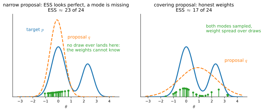
The accuracy of the estimator depends on where the proposal places its draws. Figure 27.4.1 shows both adequate and inadequate proposal coverage.
The standard health check is the weight effective sample size
\[ N_{\mathrm{eff}}=\frac{1}{\sum_{s=1}^N\bar w_s^2}, \qquad \bar w_s=\frac{w_s}{\sum_r w_r}, \tag{27.4.4}\]
which lies between \(1\) (one draw carries everything) and \(N\) (all draws count equally) and measures how concentrated the weights are. Figure 27.4.1 is a warning about its limits: the left panel’s ESS is excellent because the proposal never found the second mode. ESS can detect weights that are unequal; it cannot detect mass that was never sampled.
On our logistic posterior we compare two Gaussian proposals: the broad prior, and the local Gaussian built from the MAP and inverse Hessian computed above (the Laplace approximation, formalized below, here playing its other standard role — as a proposal generator).
def gaussian_logpdf(samples, mean, cov):
    diff = samples - mean
    sign, logdet = np.linalg.slogdet(cov)
    precision = np.linalg.inv(cov)
    return -0.5 * (len(mean) * np.log(2 * np.pi) + logdet
                   + np.einsum('ni,ij,nj->n', diff, precision, diff))

def importance(proposal_mean, proposal_cov, n, seed):
    local_rng = np.random.default_rng(seed)
    samples = local_rng.multivariate_normal(proposal_mean, proposal_cov, n)
    logw = log_joint(samples) - gaussian_logpdf(
        samples, proposal_mean, proposal_cov)
    weight = np.exp(logw - logw.max())
    weight /= weight.sum()
    mean = weight @ samples
    predictive = weight @ sigmoid(samples @ Z_new.T)
    ess = 1.0 / (weight @ weight)
    return mean, predictive, ess, weight.max()

prior_is = importance(np.zeros(2), prior_var * np.eye(2), 20000, 2)
laplace_is = importance(theta_map, laplace_cov, 5000, 3)
for name, result, n in [('prior proposal', prior_is, 20000),
                        ('Laplace proposal', laplace_is, 5000)]:
    mean, pred, ess, max_weight = result
    print(f'{name:18s}: ESS={ess:7.1f}/{n}, max weight={max_weight:.4f}, '
          f'mean={mean.round(4)}')
prior proposal : ESS= 681.1/20000, max weight=0.0029, mean=[-0.3415 1.4898]
Laplace proposal : ESS= 4287.3/5000, max weight=0.0025, mean=[-0.3359 1.4772]The prior proposal spends most of its 20,000 draws where the posterior is negligible — that is what its low ESS is reporting — while the Laplace proposal, aimed at the posterior, extracts more usable information from a quarter as many draws. This posterior is unimodal and nearly Gaussian, so the local proposal works well here. In high dimension or under mode or tail mismatch, the weights may degenerate rapidly; weight moments and effective sample size, not the nominal draw count, determine the accuracy.
27.4.3 Markov Chain Monte Carlo
Importance sampling depends on a global proposal that covers the posterior. Markov chain Monte Carlo instead constructs a Markov chain whose stationary distribution is the posterior. After convergence, dependent states from the chain can be averaged to approximate Equation 27.4.1. The Metropolis–Hastings construction needs posterior ratios between the current and proposed states, so the unknown normalizer cancels.
The Metropolis rule is easiest to state for a symmetric proposal. From \(\boldsymbol\theta\), propose \(\boldsymbol\theta'\sim q(\cdot\mid\boldsymbol\theta)\). If \(\widetilde p(\boldsymbol\theta')\ge\widetilde p(\boldsymbol\theta)\), accept the proposal; otherwise, accept it with probability \(\widetilde p(\boldsymbol\theta')/\widetilde p(\boldsymbol\theta)\) — otherwise stay put. In general, with an asymmetric proposal,
\[ \alpha(\boldsymbol\theta,\boldsymbol\theta') =\min\!\left(1, \frac{\widetilde p(\boldsymbol\theta') q(\boldsymbol\theta\mid\boldsymbol\theta')} {\widetilde p(\boldsymbol\theta) q(\boldsymbol\theta'\mid\boldsymbol\theta)}\right). \tag{27.4.5}\]
The acceptance ratio enforces detailed balance: under the target distribution, the probability flow from \(\boldsymbol\theta\) to \(\boldsymbol\theta'\) equals the reverse flow. The target posterior is therefore a stationary distribution of the chain. Convergence from an initial state also requires irreducibility, aperiodicity, and the appropriate recurrence conditions on general state spaces.
A rejection leaves the chain at its current state, so repeated states must be included when computing averages. The target normalizer is unnecessary because it cancels from the acceptance ratio.
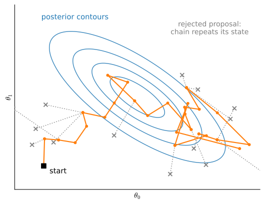
The cell runs four chains from dispersed starts, using the Laplace covariance only to scale and orient the proposal — the Metropolis correction, not that Gaussian, determines the stationary distribution.
def metropolis(start, proposal_chol, n_steps, seed):
    local_rng = np.random.default_rng(seed)
    current = np.array(start, dtype=float)
    current_logp = log_joint(current)
    draws = np.empty((n_steps, 2))
    accepted = 0
    for t in range(n_steps):
        proposal = current + proposal_chol @ local_rng.standard_normal(2)
        proposal_logp = log_joint(proposal)
        if np.log(local_rng.random()) < proposal_logp - current_logp:
            current, current_logp = proposal, proposal_logp
            accepted += 1
        draws[t] = current
    return draws, accepted / n_steps

starts = np.array([[-2.0, 0.0], [1.0, 0.3], [-1.0, 2.5], [1.0, 2.5]])
proposal_chol = 1.1 * np.linalg.cholesky(laplace_cov)
chains = []
for c, start in enumerate(starts):
    chain, accept_rate = metropolis(start, proposal_chol, 12000, 20 + c)
    chains.append(chain[2000:])                 # discard the initial transient
    print(f'chain {c + 1}: acceptance rate={accept_rate:.3f}')
chains = np.asarray(chains)
chain 1: acceptance rate=0.525
chain 2: acceptance rate=0.526
chain 3: acceptance rate=0.526
chain 4: acceptance rate=0.52727.4.3.1 Diagnosing Markov Chain Mixing
Exploration introduces dependence: consecutive states are correlated, so a chain of \(10{,}000\) states holds far less information than \(10{,}000\) independent draws — how much less depends on how fast the walk forgets where it was. Because the chain also starts wherever we put it, we need evidence that it has both forgotten its start and slowed to the right pace. Three checks answer different questions:
- Trace plots reveal sticking, drift, and chains that disagree — the failures visible to the naked eye.
- Split \(\widehat R\) compares within-chain and between-chain variation; values near one are necessary (not sufficient) for convergence: if chains from dispersed starts still disagree, none of them can be trusted.
- Effective sample size converts autocorrelation into an equivalent draw count: with autocorrelation time \(\tau=1+2\sum_{k\ge1}\rho_k\), \(M\) chains of length \(N\) contain about \(MN/\tau\) draws’ worth of information, and the Monte Carlo standard error of a posterior mean is roughly the posterior standard deviation over \(\sqrt{N_{\mathrm{eff}}}\).
The implementations below are intentionally transparent teaching versions; production software uses rank-normalized split \(\widehat R\), bulk and tail ESS, and more careful truncation of the autocorrelation sum.
def split_rhat(x):
    m, n, d = x.shape
    half = n // 2
    split = np.concatenate([x[:, :half], x[:, half:2 * half]], axis=0)
    within = split.var(axis=1, ddof=1).mean(axis=0)
    between = half * split.mean(axis=1).var(axis=0, ddof=1)
    variance = (half - 1) * within / half + between / half
    return np.sqrt(variance / within)

def autocorrelation(x):
    x = x - x.mean()
    n = len(x)
    spectrum = np.fft.rfft(x, n=2 * n)
    acov = np.fft.irfft(spectrum * np.conj(spectrum))[:n]
    return acov / acov[0]

def teaching_ess(x):
    m, n, d = x.shape
    result = []
    for j in range(d):
        rho = np.mean([autocorrelation(x[c, :, j]) for c in range(m)], axis=0)
        positive_pairs = 0.0
        for lag in range(1, n - 1, 2):
            pair = rho[lag] + rho[lag + 1]
            if pair < 0:
                break
            positive_pairs += pair
        result.append(m * n / (1 + 2 * positive_pairs))
    return np.asarray(result)

d2l.use_svg_display()
flat_chains = chains.reshape(-1, 2)
rhat = split_rhat(chains)
ess = teaching_ess(chains)
mcmc_mean = flat_chains.mean(axis=0)
mcmc_sd = flat_chains.std(axis=0, ddof=1)
print('split R-hat:', rhat.round(4))
print('ESS        :', ess.round(0).astype(int))
print('MCMC mean  :', mcmc_mean.round(4),
      '  grid mean:', posterior_mean.round(4))
print('MCSE       :', (mcmc_sd / np.sqrt(ess)).round(4))

fig, axes = d2l.plt.subplots(1, 2, figsize=(10, 3.2))
for c in range(len(chains)):
    axes[0].plot(chains[c, :600, 1], linewidth=0.8, alpha=0.8)
axes[0].set(xlabel='post-warmup iteration', ylabel=r'slope $\theta_1$',
            title='four chain traces')
for c in range(len(chains)):
    axes[1].plot(autocorrelation(chains[c, :, 1])[:80], alpha=0.8)
axes[1].axhline(0, color='black', linewidth=0.7)
axes[1].set(xlabel='lag', ylabel='autocorrelation', title='serial dependence')
d2l.plt.tight_layout()
d2l.plt.show()split R-hat: [1.0008 1.0004]
ESS : [4521 4098]
MCMC mean : [-0.3317 1.4768] grid mean: [-0.3335 1.4794]
MCSE : [0.005 0.0044]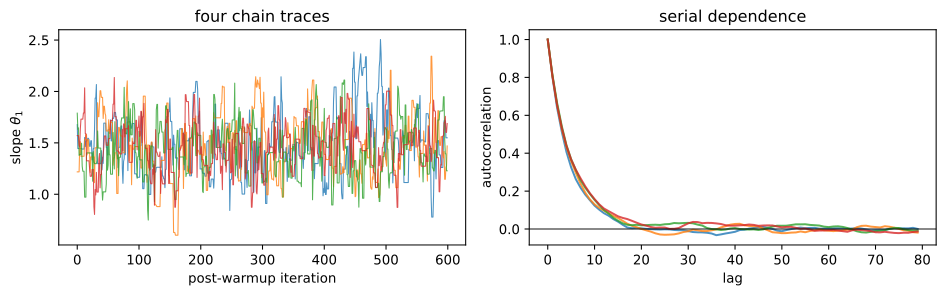
split R-hat: [1.0008 1.0004]
ESS        : [4521 4098]
MCMC mean  : [-0.3317  1.4768]   grid mean: [-0.3335  1.4794]
MCSE       : [0.005  0.0044]
split R-hat: [1.0008 1.0004]
ESS        : [4521 4098]
MCMC mean  : [-0.3317  1.4768]   grid mean: [-0.3335  1.4794]
MCSE       : [0.005  0.0044]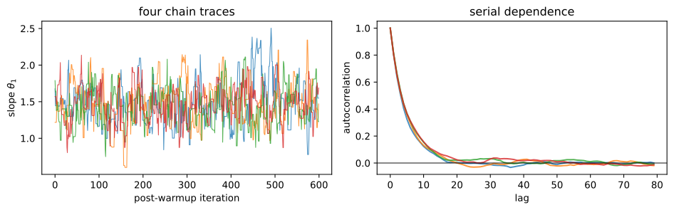
split R-hat: [1.0008 1.0004]
ESS        : [4521 4098]
MCMC mean  : [-0.3317  1.4768]   grid mean: [-0.3335  1.4794]
MCSE       : [0.005  0.0044]
Acceptance rate alone does not establish convergence. Proposals that are too small have high acceptance but strong serial correlation, while proposals that are too large are usually rejected. Extending warm-up does not correct poor mixing. Use multiple chains, inspect diagnostics for the quantities of interest, and report effective sample size and Monte Carlo error with posterior estimates.
Metropolis is a basic MCMC method. Gibbs sampling applies when conditional distributions are tractable and updates one variable or block at a time. Hamiltonian Monte Carlo uses gradients of the log posterior to propose distant states while maintaining high acceptance; the No-U-Turn Sampler adapts the trajectory length. These methods still require multiple chains, appropriate tuning, and convergence diagnostics.
27.4.4 Deterministic Approximations
Sampling represents a posterior by draws and therefore incurs Monte Carlo cost when expectations are estimated. Deterministic approximations instead replace the posterior by a tractable distribution \(q\). Laplace approximation and variational inference use different criteria for choosing \(q\) and draw on optimization (Section 27.3), Taylor expansion, and the evidence lower bound.
27.4.4.1 The Laplace Approximation at a Posterior Mode
The Laplace approximation uses a second-order expansion of the log posterior around \(\boldsymbol\theta_{\mathrm{MAP}}\). The linear term vanishes at the mode, leaving a local quadratic form. Exponentiating this quadratic gives a Gaussian. If \(H\) is the negative Hessian at the mode,
\[ p(\boldsymbol\theta\mid\mathcal D) \approx\mathcal N(\boldsymbol\theta_{\mathrm{MAP}},H^{-1}), \tag{27.4.6}\]
Computing this approximation requires the posterior mode and its Hessian. For large neural networks, the Hessian is commonly approximated by a diagonal, Kronecker-factored, or last-layer matrix to reduce computational cost.
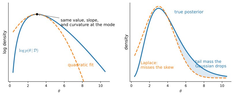
Figure 27.4.3 shows the scope of the approximation. It preserves the mode and local curvature but cannot represent skewness, heavy tails, boundaries, or additional modes. In this example, the Gaussian mean is the MAP estimate, while the exact posterior mean differs slightly because the posterior is skewed.
27.4.4.2 Variational Inference as Optimization
The Laplace approximation determines a Gaussian from local curvature at the mode. Variational inference instead chooses \(q_\phi\) from a tractable family by minimizing \(D_{\mathrm{KL}}(q_\phi\|p(\cdot\mid\mathcal D))\). The unknown evidence in this divergence is constant with respect to \(\phi\), so the equivalent optimization maximizes the ELBO
\[ \mathcal L(\phi) =\mathbb E_{q_\phi} [\log p(\mathcal D,\boldsymbol\theta)-\log q_\phi(\boldsymbol\theta)] \le\log p(\mathcal D) \tag{27.4.7}\]
Every term in this objective is computable. Optimizing a distributional approximation in this way is central to modern approximate inference. When \(q_\phi\) is produced by a neural network, the same objective trains a variational autoencoder; related variational bounds also appear in diffusion models.
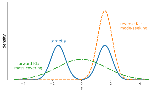
The direction of the KL divergence affects the approximation, as shown in Figure 27.4.4. Reverse KL assigns an infinite penalty when \(q\) puts mass where \(p\) is zero. If a unimodal family approximates a multimodal target, its optimum may therefore concentrate on one mode and underestimate uncertainty. Forward KL, used in moment-matching methods, instead favors covering the target mass and may place density between modes. Standard variational inference minimizes reverse KL and consequently tends toward the first behavior.
The reparameterization estimator from Section 25.4.5.1.1 supplies gradients of the ELBO. For a mean-field Gaussian \(q=\mathcal N(\mathbf m,\operatorname{diag}(\mathbf s^2))\), write \(\boldsymbol\theta=\mathbf m+\mathbf s\odot\boldsymbol\epsilon\) with \(\boldsymbol\epsilon\sim\mathcal N(\mathbf0,\mathbf I)\). Differentiation can then pass through \(\boldsymbol\theta\):
\[ \nabla_{\mathbf m}\mathcal L =\mathbb E[\nabla_{\boldsymbol\theta}\log p(\mathcal D,\boldsymbol\theta)], \qquad \nabla_{\log\mathbf s}\mathcal L =\mathbb E[\nabla_{\boldsymbol\theta}\log p \odot\mathbf s\odot\boldsymbol\epsilon]+\mathbf1, \]
where \(+\mathbf1\) is the derivative of the Gaussian entropy. The following NumPy implementation estimates these expectations with batches of 256 samples and optimizes the parameters with Adam.
rng_vi = np.random.default_rng(31)
m_vi = theta_map.copy()
log_s_vi = np.log(np.sqrt(np.diag(laplace_cov)))
m1 = np.zeros(2); v1 = np.zeros(2)
m2 = np.zeros(2); v2 = np.zeros(2)
for t in range(1, 1501):
    eps = rng_vi.standard_normal((256, 2))
    s_vi = np.exp(log_s_vi)
    theta_vi = m_vi + eps * s_vi
    grad_theta = grad_log_joint(theta_vi)
    grad_m = grad_theta.mean(axis=0)
    grad_log_s = (grad_theta * eps * s_vi).mean(axis=0) + 1.0
    for grad, param, first, second in [
            (grad_m, m_vi, m1, v1), (grad_log_s, log_s_vi, m2, v2)]:
        first *= 0.9
        first += 0.1 * grad
        second *= 0.999
        second += 0.001 * grad**2
        first_hat = first / (1 - 0.9**t)
        second_hat = second / (1 - 0.999**t)
        param += 0.03 * first_hat / (np.sqrt(second_hat) + 1e-8)

vi_cov = np.diag(np.exp(2 * log_s_vi))
print('method       mean                 marginal sd')
print('grid      ', posterior_mean.round(4), np.sqrt(np.diag(posterior_cov)).round(4))
print('Laplace   ', theta_map.round(4), np.sqrt(np.diag(laplace_cov)).round(4))
print('mean-field', m_vi.round(4), np.exp(log_s_vi).round(4))
method mean marginal sd
grid [-0.3335 1.4794] [0.3353 0.2871]
Laplace [-0.3134 1.4039] [0.3256 0.2746]
mean-field [-0.2958 1.4816] [0.3233 0.2733]The results exhibit both limitations. A diagonal mean-field covariance cannot represent posterior correlation between the intercept and slope. Reverse KL also produces a distribution that is slightly too concentrated. Full-covariance Gaussians, normalizing flows, or mixtures can represent richer dependence at greater computational and implementation cost. Convergence of the ELBO only indicates that optimization has stabilized within the chosen family; it does not establish that the family approximates the posterior well.
The following plot compares the grid reference, Metropolis draws, and the two Gaussian approximations on the same axes.
def covariance_ellipse(mean, cov, color, label):
    values, vectors = np.linalg.eigh(cov)
    angle = np.linspace(0, 2 * np.pi, 240)
    circle = np.stack([np.cos(angle), np.sin(angle)])
    ellipse = mean[:, None] + vectors @ (2 * np.sqrt(values)[:, None] * circle)
    d2l.plt.plot(ellipse[0], ellipse[1], color=color, linewidth=2, label=label)

d2l.plt.figure(figsize=(6, 4.5))
levels = np.quantile(grid_weight, [0.70, 0.90, 0.97, 0.995])
d2l.plt.contour(B0, B1, grid_weight.reshape(B0.shape),
                levels=np.unique(levels), colors='black', linewidths=1)
d2l.plt.scatter(flat_chains[::80, 0], flat_chains[::80, 1], s=5, alpha=0.15,
                label='Metropolis draws')
covariance_ellipse(theta_map, laplace_cov, 'tab:orange', 'Laplace: 2 sd')
covariance_ellipse(m_vi, vi_cov, 'tab:blue', 'mean-field VI: 2 sd')
d2l.plt.scatter(*posterior_mean, marker='x', s=70, color='black',
                label='grid mean')
d2l.plt.xlabel(r'intercept $\theta_0$')
d2l.plt.ylabel(r'slope $\theta_1$')
d2l.plt.legend(fontsize=8)
d2l.plt.tight_layout()
d2l.plt.show()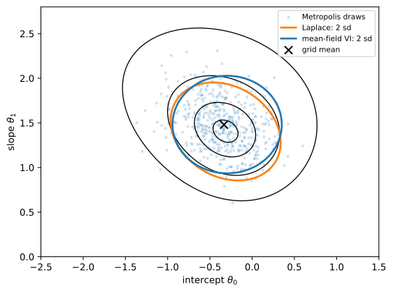
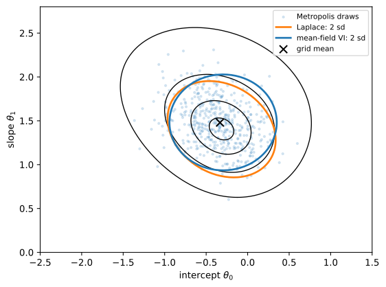
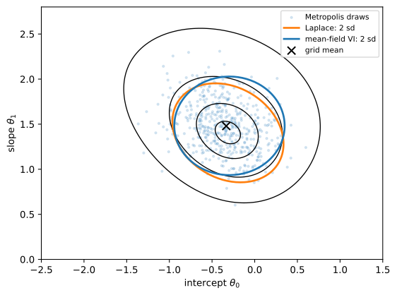
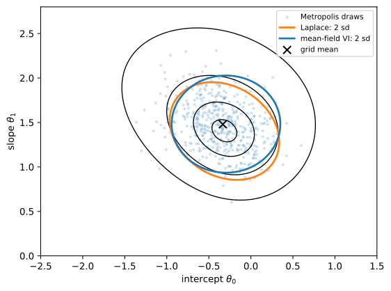
The Metropolis cloud traces the exact contours, skew included; the Laplace ellipse is centered at the MAP with roughly the right shape; the mean-field ellipse is axis-aligned — it cannot tilt — and slightly small. One plot, all four trade-offs.
27.4.5 Choosing an Approximation Method
The methods answer the same question with different failure modes.
| Method | Representation | Main diagnostic | Characteristic failure |
|---|---|---|---|
| Conjugacy / exact algebra | closed-form distribution | algebra and numerical checks | available only for special model–prior pairs |
| Grid / quadrature | weighted deterministic points | resolution and domain expansion | exponential cost in dimension |
| Importance sampling | independent weighted draws | weight ESS, largest weights, repeated runs | proposal misses or barely covers posterior mass |
| MCMC | dependent posterior draws | traces, split \(\widehat R\), ESS, MCSE | poor mixing, undiscovered modes, bad geometry |
| Laplace | one local Gaussian | comparison with samples or sensitivity to mode | skewness, tails, boundaries, multiple modes |
| Variational inference | optimized tractable \(q_\phi\) | ELBO, repeated starts, predictive checks | family restriction and local optima; biased uncertainty |
A robust workflow starts with the estimand: posterior mean, predictive probability, tail event, or decision. Use exact conjugacy when available; use a grid only as a low-dimensional check. For MCMC, run multiple chains and budget by ESS rather than iterations. For importance sampling, inspect weights. For Laplace and VI, test the approximation on posterior predictive quantities and, when feasible, compare a subset against MCMC. No scalar diagnostic proves that an unseen mode does not exist — Figure 27.4.1 is this notebook’s standing reminder.
27.4.6 Summary
- Bayesian prediction averages over the posterior and therefore represents parameter uncertainty under the specified likelihood, prior, and inference method. This does not guarantee empirical calibration; calibration must be checked on relevant data. In the logistic example, the plug-in predictions are more extreme, but that behavior is not universal.
- All four methods use evaluations of the unnormalized posterior; some variants also use its gradient. The unknown normalizer cancels — in importance ratios, in Metropolis acceptances, in the ELBO.
- Importance sampling reweights draws from a tractable proposal. Support is necessary, while tail behavior and finite moments govern variance; weight ESS cannot detect mass that was never sampled.
- Metropolis uses an acceptance ratio that establishes detailed balance. Under the convergence conditions stated above, long-run occupation follows posterior mass. Judge chains by mixing (traces, split \(\widehat R\), ESS, MCSE), never by acceptance rate alone.
- Laplace uses local value and curvature at the MAP estimate, so it misses skewness, tails, and other modes. Variational inference turns integration into optimization of the ELBO and inherits reverse KL’s mode-seeking, too-confident failure mode.
27.4.7 Exercises
- Change the prior standard deviation from \(2\) to \(0.5\) and \(10\). Compare the MAP, posterior mean, covariance, posterior predictive, and importance-sampling ESS. Which quantities are most sensitive at this sample size?
- Deliberately use an importance proposal with covariance \(0.05I\). Run ten seeds. Although this Gaussian has full mathematical support, explain why a plausible estimate in one run does not repair its poor finite-sample coverage of the posterior.
- Sweep the Metropolis proposal multiplier over \(\{0.05,0.2,0.5,1.1,3,10\}\). Plot acceptance rate against ESS per log-joint evaluation and explain why maximizing acceptance is the wrong objective.
- Replace the mean-field variational family by a full-covariance Gaussian parameterized by a Cholesky factor. Derive a valid parameterization with positive diagonal and compare the fitted correlation with the grid value.
- Create a bimodal one-dimensional posterior by using a likelihood invariant under \(\theta\mapsto-\theta\). Show how a local Laplace approximation, mean-field reverse-KL optimization, and poorly initialized MCMC can each report only one mode. Which diagnostics reveal the problem, and which do not?