%matplotlib inline
from d2l import torch as d2l
from IPython import display
import copy
import math
import torch
from torch import nn9.8 Schedules
An optimizer specifies a descent direction, a step size over time, and a method for handling gradient noise. This section studies the second choice. A learning-rate schedule maps training time \(t\) to the rate \(\eta_t\) used at that time. It can be changed independently of the remaining training loop and can substantially affect final accuracy.
Two facts force the schedule to exist, and both are already on the table. First, with a constant learning rate SGD does not converge: it reaches a noise floor proportional to \(\eta\) and rattles there indefinitely (Section 9.3). To finish well, the learning rate must come down. Second, the rate we ultimately want to train at is often not survivable at initialization: the first steps at the target rate can destroy the model before learning begins, so the learning rate must first come up. Between those two constraints — start below the target, end near zero — lies a family of shapes.
Theory ranks few of these shapes. Section 26.2.4 collects the results that do exist: the noise-floor computation, the Robbins–Monro conditions, the minimax optimality of a well-chosen constant rate for a fixed budget. None of them separates cosine decay from linear decay on a deep network. So this section proceeds the way the field does: empirically. We fix one small network and one dataset, then train the same model under one schedule after another: the classical decay shapes, then warmup, then the warmup–stable–decay schedule that large-model training adopted in the 2020s. We end with what is settled and what is not.
9.8.1 A Testbed
We need a problem cheap enough to train dozens of times and honest enough to show schedule effects. A LeNet-style convolutional network on Fashion-MNIST (Chapter 6) fits: a few seconds per epoch, yet real minibatch noise, real overfitting, and a real stability ceiling. We apply the small standard modernizations: ReLU activations, max-pooling, and batch normalization (Section 7.3) after every hidden layer. We also pin the initialization to Xavier (Section 4.4.2.2) in both frameworks. Neither choice is cosmetic. Without normalization this network’s survivable learning-rate range is narrow and seed-dependent: near its edge, identical settings live or die by initialization and data-order luck, and every comparison below would be a coin flip. And PyTorch and Flax draw different default initializations, so with defaults left in place the two framework tabs would disagree exactly where this section looks.
%matplotlib inline
from d2l import jax as d2l
from IPython import display
from flax import nnx
import jax
from jax import numpy as jnp
import math
import numpy as np
import optax
The training function takes the scheduler as an argument. At the start of every epoch it asks the scheduler for that epoch’s learning rate and installs it in the optimizer; the remaining code is the standard classification loop.
Two conventions make the runs below comparable. The training loss and the accuracies go on separate panels, since a loss near \(0.3\) and an accuracy near \(0.9\) do not belong on one scale; and we fix the random seed before building each network, so every run starts from the identical initialization and what differs between runs is the schedule, not the draw.
class SchedulerBoard:
    """Two-panel training board: loss on the left axis, accuracy on the
    right, so the two scales are not conflated on one axis. The interface
    mirrors d2l.Animator: add(x, (loss, train_acc, test_acc))."""
    def __init__(self, xlim, xlabel='epoch'):
        d2l.use_svg_display()
        self.fig, self.axes = d2l.plt.subplots(
            1, 2, figsize=(7, 2.5), constrained_layout=True)
        self.xlim, self.xlabel = xlim, xlabel
        self.X = [[] for _ in range(3)]
        self.Y = [[] for _ in range(3)]

    def add(self, x, ys):
        for i, y in enumerate(ys):
            if y is not None:
                self.X[i].append(x)
                self.Y[i].append(y)
        self.axes[0].cla()
        self.axes[0].plot(self.X[0], self.Y[0], '-')
        d2l.set_axes(self.axes[0], self.xlabel, 'loss', self.xlim, None,
                     'linear', 'linear', ['train loss'])
        self.axes[1].cla()
        self.axes[1].plot(self.X[1], self.Y[1], 'm--')
        self.axes[1].plot(self.X[2], self.Y[2], 'g-.')
        d2l.set_axes(self.axes[1], self.xlabel, 'accuracy', self.xlim, None,
                     'linear', 'linear', ['train acc', 'test acc'])
        display.display(self.fig)
display.clear_output(wait=True)Installing the rate is one assignment to trainer.param_groups. PyTorch ships the schedules of this section (and many more) in torch.optim.lr_scheduler; we write ours as plain callables to keep the mechanics visible.
The learning rate enters the jitted training step as an array argument, so changing it every epoch triggers no recompilation; the optimizer itself is constructed once with a unit rate and the update is pre-scaled. Optax ships the schedules of this section (and many more) in optax.schedules; we write ours as plain callables to keep the mechanics visible.
def net_fn():
    model = nn.Sequential(
        nn.Conv2d(1, 6, kernel_size=5, padding=2), nn.BatchNorm2d(6),
        nn.ReLU(),
        nn.MaxPool2d(kernel_size=2, stride=2),
        nn.Conv2d(6, 16, kernel_size=5), nn.BatchNorm2d(16), nn.ReLU(),
        nn.MaxPool2d(kernel_size=2, stride=2),
        nn.Flatten(),
        nn.Linear(16 * 5 * 5, 120), nn.BatchNorm1d(120), nn.ReLU(),
        nn.Linear(120, 84), nn.BatchNorm1d(84), nn.ReLU(),
        nn.Linear(84, 10))
    def init_weights(m):
        if type(m) in (nn.Linear, nn.Conv2d):
            nn.init.xavier_uniform_(m.weight)
    model.apply(init_weights)
    return model

loss = nn.CrossEntropyLoss()
device = d2l.try_gpu()

batch_size = 256
train_iter, test_iter = d2l.load_data_fashion_mnist(batch_size=batch_size)

def train(net, train_iter, test_iter, num_epochs, loss, trainer, device,
          scheduler=None, animator=None, epoch_offset=0):
    net.to(device)
    if animator is None:
        animator = SchedulerBoard(xlim=[0, num_epochs])
    for epoch in range(num_epochs):
        if scheduler:
            for param_group in trainer.param_groups:
                param_group['lr'] = scheduler(epoch)
        net.train()
        metric = d2l.Accumulator(3)  # train_loss, train_acc, num_examples
        for i, (X, y) in enumerate(train_iter):
            trainer.zero_grad()
            X, y = X.to(device), y.to(device)
            y_hat = net(X)
            l = loss(y_hat, y)
            l.backward()
            trainer.step()
            with torch.no_grad():
                metric.add(l * X.shape[0], d2l.accuracy(y_hat, y), X.shape[0])
            train_loss = metric[0] / metric[2]
            train_acc = metric[1] / metric[2]
            if (i + 1) % 50 == 0:
                animator.add(epoch_offset + epoch + i / len(train_iter),
                             (train_loss, train_acc, None))
        test_acc = d2l.evaluate_accuracy_gpu(net, test_iter)
        animator.add(epoch_offset + epoch + 1, (None, None, test_acc))
    print(f'train loss {train_loss:.3f}, train acc {train_acc:.3f}, '
          f'test acc {test_acc:.3f}')
xavier = nnx.initializers.xavier_uniform()
class Net(nnx.Module):
def __init__(self, rngs=None):
rngs = nnx.Rngs(0) if rngs is None else rngs
self.conv1 = nnx.Conv(1, 6, kernel_size=(5, 5), padding='same',
kernel_init=xavier, rngs=rngs)
self.bn1 = nnx.BatchNorm(6, rngs=rngs)
self.conv2 = nnx.Conv(6, 16, kernel_size=(5, 5), padding='valid',
kernel_init=xavier, rngs=rngs)
self.bn2 = nnx.BatchNorm(16, rngs=rngs)
self.fc1 = nnx.Linear(16 * 5 * 5, 120, kernel_init=xavier, rngs=rngs)
self.bn3 = nnx.BatchNorm(120, rngs=rngs)
self.fc2 = nnx.Linear(120, 84, kernel_init=xavier, rngs=rngs)
self.bn4 = nnx.BatchNorm(84, rngs=rngs)
self.fc3 = nnx.Linear(84, 10, kernel_init=xavier, rngs=rngs)
def __call__(self, x):
x = nnx.max_pool(nnx.relu(self.bn1(self.conv1(x))),
window_shape=(2, 2), strides=(2, 2))
x = nnx.max_pool(nnx.relu(self.bn2(self.conv2(x))),
window_shape=(2, 2), strides=(2, 2))
x = x.reshape((x.shape[0], -1))
x = nnx.relu(self.bn3(self.fc1(x)))
x = nnx.relu(self.bn4(self.fc2(x)))
return self.fc3(x)
def net_fn():
return Net()
loss_fn = optax.softmax_cross_entropy_with_integer_labels
batch_size = 256
data = d2l.FashionMNIST(batch_size=batch_size)
train_iter = data.get_dataloader(train=True)
test_iter = data.get_dataloader(train=False)
def evaluate_accuracy_jax(model, data_iter):
@nnx.jit
def eval_step(model, X, y):
y_hat = model(X)
return jnp.array([jnp.sum(jnp.argmax(y_hat, axis=1) == y),
y.shape[0]])
model.eval() # use running averages in the BatchNorm layers
metric = jnp.zeros(2) # num_correct, num_examples
for X, y in data_iter:
X, y = jnp.array(X), jnp.array(y)
metric += eval_step(model, X, y)
return float(metric[0] / metric[1])
def train(net, train_iter, test_iter, num_epochs, lr, scheduler=None,
animator=None, epoch_offset=0):
model = net if isinstance(net, nnx.Module) else net()
# One optimizer for the entire run. The scalar learning rate is an array
# argument to the compiled step, so changing it does not recompile.
optimizer = nnx.Optimizer(model, optax.sgd(1.0), wrt=nnx.Param)
@nnx.jit
def train_step(model, optimizer, X, y, learning_rate):
def compute_loss(model):
logits = model(X)
loss = jnp.mean(loss_fn(logits, y))
correct = jnp.sum(jnp.argmax(logits, axis=1) == y)
return loss, correct
(l, correct), grads = nnx.value_and_grad(
compute_loss, has_aux=True)(model)
grads = jax.tree.map(lambda g: learning_rate * g, grads)
optimizer.update(model, grads)
return jnp.array([l * X.shape[0], correct, X.shape[0]])
if animator is None:
animator = SchedulerBoard(xlim=[0, num_epochs])
num_batches = len(train_iter)
for epoch in range(num_epochs):
model.train()
metric = jnp.zeros(3) # train_loss, train_correct, num_examples
learning_rate = jnp.asarray(scheduler(epoch) if scheduler else lr)
for i, (X, y) in enumerate(train_iter):
X, y = jnp.array(X), jnp.array(y)
metric += train_step(model, optimizer, X, y, learning_rate)
if (i + 1) % 50 == 0:
train_loss, train_acc = np.asarray(
metric[:2] / metric[2]).tolist()
animator.add(epoch_offset + epoch + i / num_batches,
(train_loss, train_acc, None))
train_loss, train_acc = np.asarray(metric[:2] / metric[2]).tolist()
test_acc = evaluate_accuracy_jax(model, test_iter)
animator.add(epoch_offset + epoch + 1, (None, None, test_acc))
print(f'train loss {train_loss:.3f}, train acc {train_acc:.3f}, '
f'test acc {test_acc:.3f}')The baseline is the schedule most code starts life with: a constant. We pick \(\eta = 0.3\) and train for 30 epochs.
lr, num_epochs = 0.3, 30
torch.manual_seed(0)
net = net_fn()
trainer = torch.optim.SGD(net.parameters(), lr=lr)
train(net, train_iter, test_iter, num_epochs, loss, trainer, device)
train loss 0.061, train acc 0.977, test acc 0.895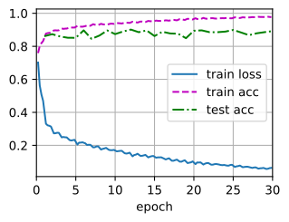
lr, num_epochs = 0.3, 30
train(net_fn, train_iter, test_iter, num_epochs, lr)
train loss 0.059, train acc 0.979, test acc 0.904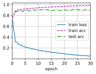
The baseline exhibits two failure modes addressed by the schedules below. The training loss stays visibly noisy to the end: the iterate is riding its noise floor, and no amount of extra training lowers it. And while training accuracy keeps climbing, test accuracy stalls after roughly ten epochs; the widening gap is overfitting. Both symptoms respond to a decaying learning rate — though, as the first attempt below shows, not to every decaying rate.
9.8.2 Decay Schedules
A scheduler here is any callable that maps the epoch index to a learning rate. Statelessness is worth insisting on: a schedule should be a function of time, not an object that remembers how often it was called, because a pure function can be plotted, resumed at epoch 17, or evaluated backwards without bookkeeping. That discipline looks pedantic now and pays off at the end of this section, when we branch new schedules off the middle of a finished run.
9.8.2.1 Square-Root Decay
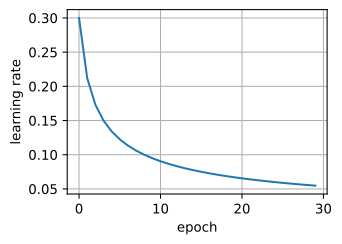
Section 9.3 established the convex baseline: with \(\eta_t = \eta_0\, (t+1)^{-1/2}\), SGD converges at the optimal rate for convex problems. That makes square-root decay the theory-first choice.
class SquareRootScheduler:
    def __init__(self, lr=0.1):
        self.lr = lr

    def __call__(self, epoch):
        return self.lr * pow(epoch + 1.0, -0.5)

scheduler = SquareRootScheduler(lr=0.3)
d2l.plot(d2l.arange(num_epochs), [scheduler(t) for t in range(num_epochs)],
         xlabel='epoch', ylabel='learning rate')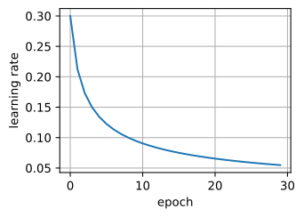
Training with it is a one-argument change.
torch.manual_seed(0)
net = net_fn()
trainer = torch.optim.SGD(net.parameters(), lr)
train(net, train_iter, test_iter, num_epochs, loss, trainer, device,
      scheduler)
train loss 0.095, train acc 0.967, test acc 0.902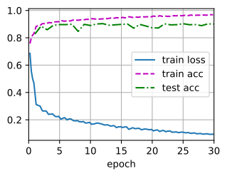
train(net_fn, train_iter, test_iter, num_epochs, lr, scheduler)train loss 0.088, train acc 0.970, test acc 0.905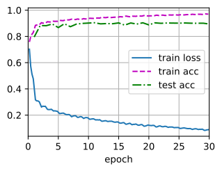
The loss curve is smoother and the late-epoch noise reduced, the noise floor shrinking as \(\eta_t\) falls. But the final test accuracy is no better than the constant baseline’s, in either framework. The diagnosis is the shape: square-root decay manages to be timid at both ends. It halves the rate within the first three epochs, giving up the large early steps that do the exploring, yet it ends the run at \(\eta_{29} \approx 0.05\), the largest final rate of any decay in this section, so it never fully quenches the noise either. Its guarantee speaks about convex problems; a neural network wants the opposite temperament. Every schedule that follows has it: stay high longer, decay harder at the end.
9.8.2.2 Multiplicative Decay
An alternative with the same monotone spirit is multiplicative (exponential) decay, \(\eta_{t+1} = \eta_t \cdot \alpha\) for some \(\alpha \in (0, 1)\), usually clipped at a floor so the rate does not vanish entirely: \(\eta_t = \max(\eta_{\min},\ \eta_0 \cdot \alpha^t)\).
class FactorScheduler:
    def __init__(self, factor=1, stop_factor_lr=1e-7, base_lr=0.1):
        self.factor = factor
        self.stop_factor_lr = stop_factor_lr
        self.base_lr = base_lr

    def __call__(self, epoch):
        return max(self.stop_factor_lr, self.base_lr * self.factor ** epoch)

scheduler = FactorScheduler(factor=0.9, stop_factor_lr=0.01, base_lr=0.3)
d2l.plot(d2l.arange(50), [scheduler(t) for t in range(50)],
         xlabel='epoch', ylabel='learning rate')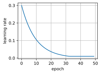
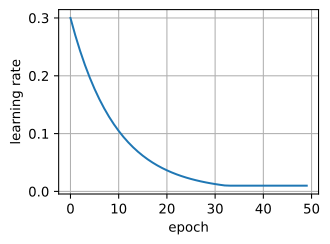
The shape differs from square root where it counts: with \(\alpha = 0.9\) the early decline is gentler, and by epoch 30 the rate has fallen more than twentyfold, compared with fivefold under square-root decay. It therefore reduces the rate much more strongly near the end. The floor guards the other edge: with \(\alpha\) too small the rate becomes negligible before the model has learned enough.
torch.manual_seed(0)
net = net_fn()
trainer = torch.optim.SGD(net.parameters(), lr)
train(net, train_iter, test_iter, num_epochs, loss, trainer, device,
      scheduler)
train loss 0.093, train acc 0.970, test acc 0.906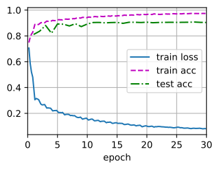
train(net_fn, train_iter, test_iter, num_epochs, lr, scheduler)train loss 0.084, train acc 0.973, test acc 0.908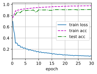
Both measured symptoms improve: the final loss fluctuates less, the test accuracy sits visibly above the constant baseline’s, and the train–test gap narrows. The remaining shapes repeat this pattern; what varies is how the high-rate budget is spent and how the descent is timed.
9.8.2.3 Piecewise Constant Decay
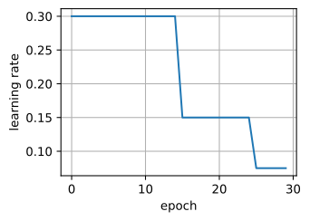
Piecewise constant decay, widely used in ImageNet training, holds the rate constant and reduces it by a fixed factor at preset epochs. This schedule matches the noise-floor analysis of Section 9.3: reduce the rate after the iterates stop improving at the current noise floor. Training curves under this schedule have a characteristic staircase shape, with a visible drop in loss right after each cut.
class MultiFactorScheduler:
    def __init__(self, milestones, factor, base_lr):
        self.milestones = milestones
        self.factor = factor
        self.base_lr = base_lr

    def __call__(self, epoch):
        lr = self.base_lr
        for milestone in self.milestones:
            if epoch >= milestone:
                lr *= self.factor
        return lr

scheduler = MultiFactorScheduler(milestones=[15, 25], factor=0.5, base_lr=0.3)
d2l.plot(d2l.arange(num_epochs), [scheduler(t) for t in range(num_epochs)],
         xlabel='epoch', ylabel='learning rate')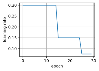
torch.manual_seed(0)
net = net_fn()
trainer = torch.optim.SGD(net.parameters(), lr)
train(net, train_iter, test_iter, num_epochs, loss, trainer, device,
      scheduler)
train loss 0.044, train acc 0.987, test acc 0.909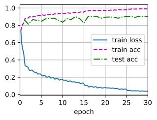
train(net_fn, train_iter, test_iter, num_epochs, lr, scheduler)train loss 0.041, train acc 0.988, test acc 0.906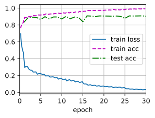
The milestones are additional hyperparameters, and their useful values depend on the budget, dataset, and architecture. Cosine decay removes these discrete transition points.
9.8.2.4 Cosine Decay
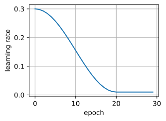
You have trained with this schedule already: the recipe of Section 7.6 combined cosine decay with warmup as standard equipment, and the models of that chapter rode it to their best accuracies. What that section took on faith, this one examines. Loshchilov and Hutter (2016) proposed the shape on the reasoning that one should not decrease the learning rate too drastically at the start and should end with a very small rate to refine the solution. For a horizon of \(T\) epochs,
\[\eta_t = \eta_T + \frac{\eta_0 - \eta_T}{2}\left(1 + \cos(\pi t/T)\right), \tag{9.8.1}\]
which glides from \(\eta_0\) to \(\eta_T\) with no kinks and only the peak rate left to tune. For \(t > T\) the rate is pinned at \(\eta_T\). The implementation below also carries an optional linear ramp over the first warmup_steps epochs; we ignore it for the moment and pick it up in the next subsection.
class CosineScheduler:
    def __init__(self, max_update, base_lr=0.01, final_lr=0,
                 warmup_steps=0, warmup_begin_lr=0):
        self.max_update = max_update
        self.base_lr = base_lr
        self.final_lr = final_lr
        self.warmup_steps = warmup_steps
        self.warmup_begin_lr = warmup_begin_lr

    def __call__(self, epoch):
        if epoch < self.warmup_steps:
            increase = (self.base_lr - self.warmup_begin_lr) \
                       * (epoch + 1) / self.warmup_steps
            return self.warmup_begin_lr + increase
        if epoch < self.max_update:
            t = (epoch - self.warmup_steps) \
                / (self.max_update - self.warmup_steps)
            return self.final_lr + (self.base_lr - self.final_lr) \
                * (1 + math.cos(math.pi * t)) / 2
        return self.final_lr

scheduler = CosineScheduler(max_update=20, base_lr=0.3, final_lr=0.01)
d2l.plot(d2l.arange(num_epochs), [scheduler(t) for t in range(num_epochs)],
         xlabel='epoch', ylabel='learning rate')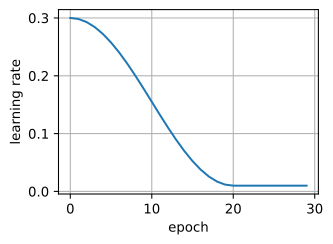
torch.manual_seed(0)
net = net_fn()
trainer = torch.optim.SGD(net.parameters(), lr)
train(net, train_iter, test_iter, num_epochs, loss, trainer, device,
      scheduler)
train loss 0.090, train acc 0.970, test acc 0.911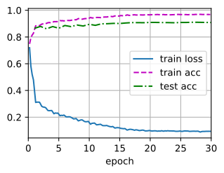
train(net_fn, train_iter, test_iter, num_epochs, lr, scheduler)train loss 0.080, train acc 0.975, test acc 0.909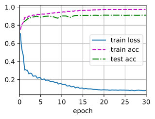
On this testbed cosine decay lands in the same accuracy range as multiplicative and piecewise constant decay — among the stay-high, decay-hard shapes the differences are too close to call from a single run, and claiming otherwise would be reading tea leaves. Cosine’s appeal is operational: one parameter, no milestones, graceful behavior across budgets. That, more than any measured superiority, is why it spread.
9.8.3 Warmup
Every schedule so far answers “how should the rate come down?”. Warmup answers a different question: how should it come up? Section 7.6 gave the operational answer: a freshly initialized network produces large, badly scaled gradients, so ramp gently. You have been warming up ever since. The mechanism deserves a closer look. At initialization the parameters are random and the loss surface around them can be sharply curved in some directions. A learning rate that the network would happily accept after a few epochs of training can be fatal in step one: the updates overshoot, and the run never recovers. Goyal et al. (2017) ran into exactly this when scaling ImageNet training to large batches and correspondingly large learning rates, and made the fix standard practice: ramp the rate linearly from near zero to the target over the first few epochs. Why this works has since been studied directly: early training at a growing rate progressively reduces the sharpness of the loss around the iterate, so the network can tolerate a target rate that would have diverged from cold (Kalra and Barkeshli 2024). Warmup does not make every rate stable, but it can raise the largest usable target rate and avoid applying that rate to the poorly scaled initial gradients. For adaptive methods such as Adam there is a second, independent reason to warm up: the preconditioner is estimated from a handful of gradients early on and should not be trusted at full step size (Section 26.2.4). Our testbed uses plain SGD, which isolates the curvature mechanism.
Batch normalization lets this network tolerate a broad range of initial learning rates, but a stability limit remains. We train at \(\eta = 7.5\), twenty-five times the baseline rate:
hot_lr = 7.5
torch.manual_seed(0)
net = net_fn()
trainer = torch.optim.SGD(net.parameters(), lr=hot_lr)
train(net, train_iter, test_iter, 10, loss, trainer, device)
train loss 2.314, train acc 0.099, test acc 0.100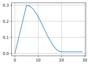
hot_lr = 7.5
train(net_fn, train_iter, test_iter, 10, hot_lr)
train loss 2.315, train acc 0.097, test acc 0.100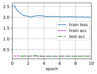
The run remains at chance accuracy after the first epoch: the loss hovers near \(\ln 10 \approx 2.3\), the loss of predicting all ten classes uniformly, and accuracy never leaves the vicinity of chance. The oversized first steps threw the parameters so far from the initialization that no useful signal survived. A five-epoch linear ramp reaches the same target rate gradually:
def warmup(epoch):
return hot_lr * min((epoch + 1) / 5, 1)torch.manual_seed(0)
net = net_fn()
trainer = torch.optim.SGD(net.parameters(), lr=hot_lr)
train(net, train_iter, test_iter, 10, loss, trainer, device, warmup)train loss 0.217, train acc 0.916, test acc 0.874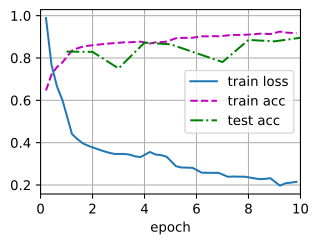
train(net_fn, train_iter, test_iter, 10, hot_lr, warmup)train loss 0.207, train acc 0.921, test acc 0.891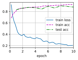
With the ramp, this fixed-seed run reaches 80–90% accuracy in ten epochs at the same target rate. Cold starts at lower rates can remain stable, while rates sufficiently above the stability limit fail even with warmup. Thus the experiment shows that warmup widens the usable range for this model; it does not remove its upper edge. Gotmare et al. (2018) probed what warmup does inside deeper networks and found its main measurable effect is exactly this kind of containment: it limits how far the parameters, especially in later layers, can diverge while the parameters and optimizer statistics remain near their initial random state.
Combining the ramp with cosine decay gives the schedule that trained most of the deep learning models of the late 2010s and remains a strong default: linear warmup to the peak, cosine decay to near zero.
scheduler = CosineScheduler(max_update=30, base_lr=0.3, final_lr=0.01,
                            warmup_steps=5)
d2l.plot(d2l.arange(num_epochs), [scheduler(t) for t in range(num_epochs)],
         xlabel='epoch', ylabel='learning rate')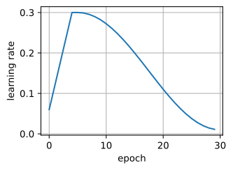
torch.manual_seed(0)
net = net_fn()
trainer = torch.optim.SGD(net.parameters(), lr)
train(net, train_iter, test_iter, num_epochs, loss, trainer, device,
      scheduler)
train loss 0.050, train acc 0.986, test acc 0.908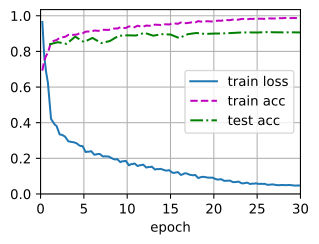
train(net_fn, train_iter, test_iter, num_epochs, lr, scheduler)train loss 0.047, train acc 0.987, test acc 0.910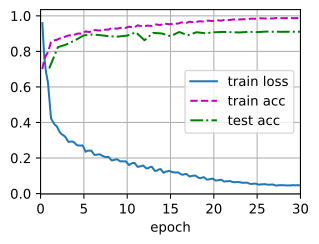
9.8.4 Warmup–Stable–Decay
Cosine decay has a defect that none of our plots show: the horizon \(T\) is baked into the schedule from step one. Every intermediate checkpoint of a cosine run is a model whose learning rate was mid-descent: fine to resume, useless as a finished product, because its rate never came down. Decide after the fact that the model should have trained for twice as long and the schedule has reached its endpoint; the available options are to retrain from scratch or to splice schedules in ways cosine was never designed for. For a single fixed-budget run this is no burden. It becomes one when the budget is unknown because data continue to arrive or the loss is still falling at \(T\). The dependence is especially restrictive when one training run must yield models at several budgets*, as in a scaling-law study (Section 9.11).
The schedule that large language model training converged on instead is warmup–stable–decay (WSD) (Hu et al. 2024): warm up, hold the peak rate constant for most of the run, and decay only in a short final phase, typically the last 10–20% of the budget. The MiniCPM team popularized it, and Hägele et al. (2024) showed that it matches cosine across budgets. The constant plateau provides this flexibility: every plateau checkpoint is a horizon-free starting point. A decay phase can be branched from such a checkpoint whenever a finished model is needed.
class WSDScheduler:
    def __init__(self, max_update, decay_steps, base_lr=0.1, final_lr=0,
                 warmup_steps=0):
        self.max_update = max_update
        self.decay_steps = decay_steps
        self.base_lr = base_lr
        self.final_lr = final_lr
        self.warmup_steps = warmup_steps

    def __call__(self, epoch):
        if epoch < self.warmup_steps:
            return self.base_lr * (epoch + 1) / self.warmup_steps
        if epoch < self.max_update - self.decay_steps:
            return self.base_lr
        t = min((epoch - (self.max_update - self.decay_steps) + 1)
                / self.decay_steps, 1)
        return self.base_lr + (self.final_lr - self.base_lr) * t

scheduler = WSDScheduler(max_update=30, decay_steps=6, base_lr=0.3,
                         final_lr=0.01, warmup_steps=5)
d2l.plot(d2l.arange(num_epochs), [scheduler(t) for t in range(num_epochs)],
         xlabel='epoch', ylabel='learning rate')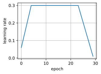
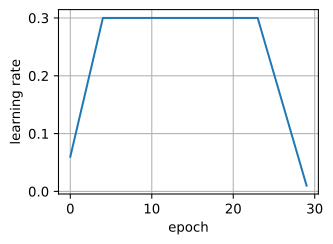
Trained at the same peak rate and the same 30-epoch budget as the warmup-plus-cosine run above, WSD lands in the same final accuracy range. Watch the shape of its loss curve rather than the endpoint: through the long plateau the training loss sits above the cosine run’s at the same epoch, then drops abruptly once the decay begins.
torch.manual_seed(0)
net = net_fn()
trainer = torch.optim.SGD(net.parameters(), lr)
train(net, train_iter, test_iter, num_epochs, loss, trainer, device,
      scheduler)
train loss 0.029, train acc 0.994, test acc 0.906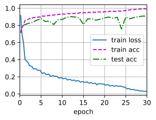
train(net_fn, train_iter, test_iter, num_epochs, lr, scheduler)train loss 0.027, train acc 0.994, test acc 0.914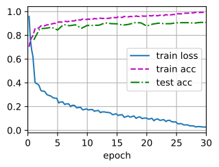
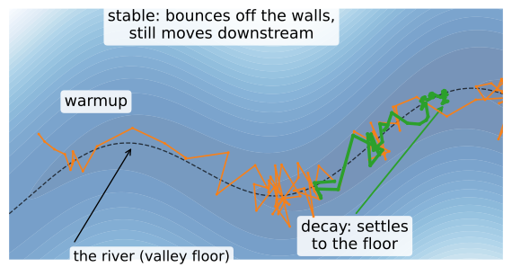
This rapid final decrease appears in published WSD loss curves, and Wen et al. (2024) give it a useful geometry. Picture the loss surface as a river valley: steep walls transverse to a floor that winds downhill at a gentle slope. At the plateau’s high learning rate the iterate bounces between the walls while drifting fast along the floor. The bouncing inflates the measured loss — the iterate is always partway up a wall — but the drift is real progress, covering distance along the valley that small steps could not match. The decay quenches the bouncing: the iterate settles to the floor it has already reached, and the loss decreases rapidly. In this interpretation, the plateau phase moves along the shallow direction and the decay phase reduces oscillation across the steep direction, which is why the plateau can be extended for as long as you keep training and why a short decay suffices. It is the noise-ball argument of Section 9.3 upgraded from a bowl to a winding valley. Figure 9.8.1 draws it: the same seeded noise drives both runs, and the only difference between bouncing forever and landing on the floor is what the learning rate does at the end.
9.8.4.1 Branching Off the Plateau
The river-valley interpretation predicts that if transverse oscillation is the main deficit of a plateau checkpoint, a decay branched off any plateau point should land it. We verify the whole WSD workflow, drawing all three runs below on one shared pair of axes over absolute epochs 0–36 so that the branch point stays visible. First train warmup-plus-stable only; this is the run an open-ended training job would be in the middle of. Its training loss hovers noisily at several times the level the decayed runs reach, and its test accuracy wanders at or below theirs: not yet a finished model.
torch.manual_seed(0)
net_plateau = net_fn()
trainer = torch.optim.SGD(net_plateau.parameters(), lr)
stable = WSDScheduler(max_update=24, decay_steps=0, base_lr=0.3,
                      warmup_steps=5)
board = SchedulerBoard(xlim=[0, 36])
train(net_plateau, train_iter, test_iter, 24, loss, trainer, device, stable,
      animator=board)
train loss 0.090, train acc 0.966, test acc 0.873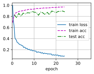
model_plateau = net_fn()
stable = WSDScheduler(max_update=24, decay_steps=0, base_lr=0.3,
                      warmup_steps=5)
board = SchedulerBoard(xlim=[0, 36])
train(model_plateau, train_iter, test_iter, 24, lr, stable, animator=board)
train loss 0.091, train acc 0.967, test acc 0.904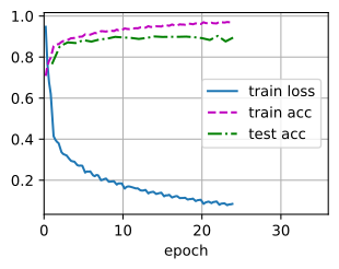
Because this run has no fixed horizon, we continue it for six more epochs at the constant peak rate.
train(net_plateau, train_iter, test_iter, 6, loss, trainer, device,
      animator=board, epoch_offset=24)
board.fig
train loss 0.065, train acc 0.977, test acc 0.892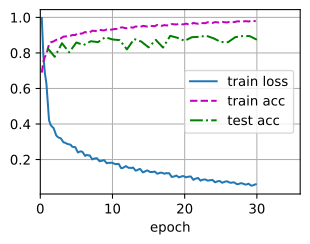
train(model_plateau, train_iter, test_iter, 6, lr, animator=board,
      epoch_offset=24)
board.fig
train loss 0.065, train acc 0.976, test acc 0.901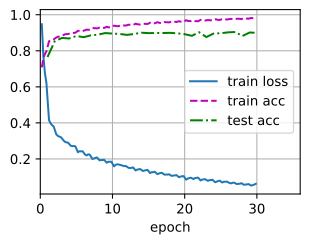
We then clone the plateau checkpoint and branch a six-epoch decay from the clone, assembling a 36-epoch WSD schedule that nobody planned when training started:
net_branch = copy.deepcopy(net_plateau)
decay = WSDScheduler(max_update=6, decay_steps=6, base_lr=0.3, final_lr=0.01)
train(net_branch, train_iter, test_iter, 6, loss,
      torch.optim.SGD(net_branch.parameters(), lr), device, decay,
      animator=board, epoch_offset=30)
board.fig
train loss 0.017, train acc 0.997, test acc 0.903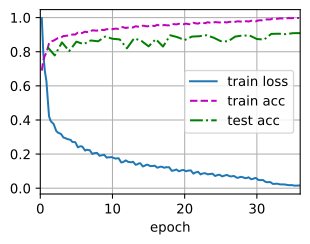
model_branch = nnx.clone(model_plateau)
decay = WSDScheduler(max_update=6, decay_steps=6, base_lr=0.3, final_lr=0.01)
train(model_branch, train_iter, test_iter, 6, lr, decay, animator=board,
      epoch_offset=30)
board.fig
train loss 0.017, train acc 0.997, test acc 0.908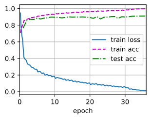
The loss decreases at epoch 30, when the decay branches from the plateau, and the branched model reaches the same accuracy range as the full cosine and WSD runs even though the horizon was not chosen in advance. This is the property that spread WSD at the frontier: one long stable run plus short branched decays yields models at many budgets for roughly the cost of one, where cosine would demand a separate full run per budget (Hägele et al. 2024). One practical note: our optimizer is plain SGD, which carries no state, so cloning the parameters was enough. With momentum or Adam, the optimizer state must be checkpointed and branched along with them.
9.8.4.2 The Current Frontier
Three developments close the section; the balance among them is a snapshot of mid-2026, and this is the corner of the chapter most likely to date.
Linear decay to zero. Defazio et al. (2023) argue from worst-case analysis that a linear decay to exactly zero is the shape to beat, and Bergsma et al. (2025) back this at LLM scale: across model sizes and budgets, warmup plus linear-to-zero matched or beat both cosine and WSD variants in their sweeps. The final rate matters more than the path taken to it; schedules that stop at a nonzero floor leave the last increment of loss on the table.
Schedule-free methods. Defazio et al. (2024) remove the schedule altogether: keep stepping at a constant rate, and evaluate a running average of the iterates rather than the latest one. The scheme is coupled rather than post-hoc: each gradient is taken at an interpolation between the fast iterate and the average, and the average is what you evaluate (the exact recurrence is in the exercises). Averaging and decay both reduce endpoint variability, but by different operations: decay changes subsequent iterates, while averaging cancels some fluctuations in the evaluated parameters. The averaged iterate can therefore provide a low-variance endpoint whose horizon is always “now”, the same operational property as WSD’s branched decays. Section 9.12 returns to weight averaging in its more common role as a cheap accuracy bump (Izmailov et al. 2018); the exercises below have you watch the schedule-free effect on a noisy quadratic.
The comparison between WSD and cosine is not settled. The GLM-4.5 team ablated both at scale and shipped cosine (Zeng et al. 2025), and at matched tuning the measured differences between modern schedules are small and consistently less than the gains from tuning the peak rate. What is settled is operational: plateau checkpoints that can be decayed on demand are strictly more flexible than a schedule that commits to its horizon at step one, and that, more than any loss-curve gap, is why WSD and its relatives became widespread where the training horizon is open-ended.
9.8.5 Summary
- A schedule is a function from training time to learning rate. Decay exists to lower SGD’s noise floor (and, empirically, the train–test gap); warmup exists because the target rate is often unsafe at initialization.
- The decay shapes disagree more in their timing than their endpoints. Square-root decay gives up the high early rate and, on our testbed, lands below the constant baseline; multiplicative, piecewise constant, and cosine decay stay high longer, quench harder at the end, improve on the baseline, and are too close to call from single runs. Cosine won on convenience: one parameter, no milestones.
- Warmup raises the stability ceiling by giving the network time to reduce sharpness before the full rate arrives. At rates where a cold start dies, a short linear ramp trains.
- Warmup–stable–decay holds the peak rate for most of the run and decays late. Its rapid final loss decrease follows from reducing stochastic fluctuations (the river-valley picture), and its plateau checkpoints can be branched into finished models at any time, which supports its use in large-scale training.
- Linear decay to zero is a strong, simple recent default; schedule-free averaging replaces decay with iterate averaging; WSD versus cosine remains genuinely contested.
9.8.6 Exercises
- Experiment with the constant baseline: train at \(\eta \in \{0.03, 0.1, 0.3, 0.5\}\). Which gives the best final test accuracy? What happens to the train–test gap as \(\eta\) shrinks?
- Implement polynomial decay \(\eta_t = \eta_0 (\beta t + 1)^{-\alpha}\). Setting \(\alpha = 0.5\) recovers square-root decay; try \(\alpha \in \{0.25, 1, 2\}\) and describe how \(\alpha\) trades early progress against late noise.
- How long should warmup last? At the target rate of this section’s demo, vary the ramp from 1 to 10 epochs. Then raise the target rate until no warmup length saves the run — the stability ceiling is real, warmup only moves it.
- Extend the plateau run of this section to 60 epochs and branch 6-epoch decays at epochs 30, 40, and 50. Plot final test accuracy against branch point. You have traced an accuracy-versus-budget curve from a single run, which is the experimental design of Hägele et al. (2024) .
- Implement schedule-free SGD (Defazio et al. 2024) on a noisy 2-D quadratic \(f(\mathbf{x}) = \frac{1}{2}\mathbf{x}^\top \mathrm{diag}(1, 10)\, \mathbf{x}\) with Gaussian gradient noise. Iterate \(\mathbf{y}_t = (1-\beta)\mathbf{z}_t + \beta \mathbf{x}_t\), \(\mathbf{z}_{t+1} = \mathbf{z}_t - \eta \nabla f(\mathbf{y}_t)\), \(\mathbf{x}_{t+1} = (1 - c_{t+1})\mathbf{x}_t + c_{t+1}\mathbf{z}_{t+1}\) with \(c_{t+1} = 1/(t+1)\) and \(\beta = 0.9\). Plot \(f(\mathbf{z}_t)\) and \(f(\mathbf{x}_t)\) over 500 steps at constant \(\eta\). The base iterate rides its noise ball; the averaged iterate keeps descending, tracking an implicit decay without ever changing \(\eta\).
- Constant-rate SGD does not converge, but its stationary noise is not useless: Welling and Teh (2011) turn it into a sampler. Read about stochastic gradient Langevin dynamics and relate the injected noise scale to the noise floor of Section 9.3.