6.1 From Fully Connected Layers to Convolutions
The models introduced so far treat the input as a collection of features without assuming a spatial relation among them. This is appropriate for many tabular datasets, where columns have no natural ordering. Images have a known two-dimensional organization, and ignoring it makes a fully connected model both inefficient and insensitive to useful prior knowledge.
Consider a classifier that distinguishes cats from dogs in one-megapixel photographs. This means that each input to the network has one million dimensions. Even an aggressive reduction to one thousand hidden dimensions would require a fully connected layer with \(10^6 \times 10^3 = 10^9\) parameters. In 32-bit floating point, the weights alone occupy 4 GB, before gradients, optimizer state, and activations are stored. The layer is therefore expensive to train and statistically difficult to estimate unless the dataset is correspondingly large.
Reducing the resolution to one hundred thousand pixels does not remove the problem, because a practical representation may also require substantially more than 1000 hidden units. A fully connected model can therefore still require billions of parameters. Moreover, learning a classifier by fitting so many parameters might require collecting an enormous dataset. And yet today both humans and computers are able to distinguish cats from dogs quite well, seemingly contradicting these intuitions. Images exhibit spatial structure that a model can exploit. Convolutional neural networks (CNNs) encode two important parts of this structure: local interactions and a shared response to the same pattern at different locations. The derivation below maps an input image \(\mathbf{X}\) to a hidden representation \(\mathbf{H}\) while imposing these two constraints.
6.1.1 Invariance
An object detector should recognize a pattern at different locations in an image. The children’s game “Where’s Waldo,” illustrated in Figure 6.1.1, provides a simple example: the target retains its identity regardless of where it appears in the scene. Each scene contains many people and activities, with Waldo placed among the distractions. His appearance does not depend on his location. A detector could therefore scan the image and assign each patch a score indicating its likelihood of containing Waldo. In fact, many object detection (Girshick et al. 2014) and semantic segmentation (Long et al. 2015) algorithms are based on this approach. CNNs systematize this idea of spatial invariance, exploiting it to learn useful representations with fewer parameters.
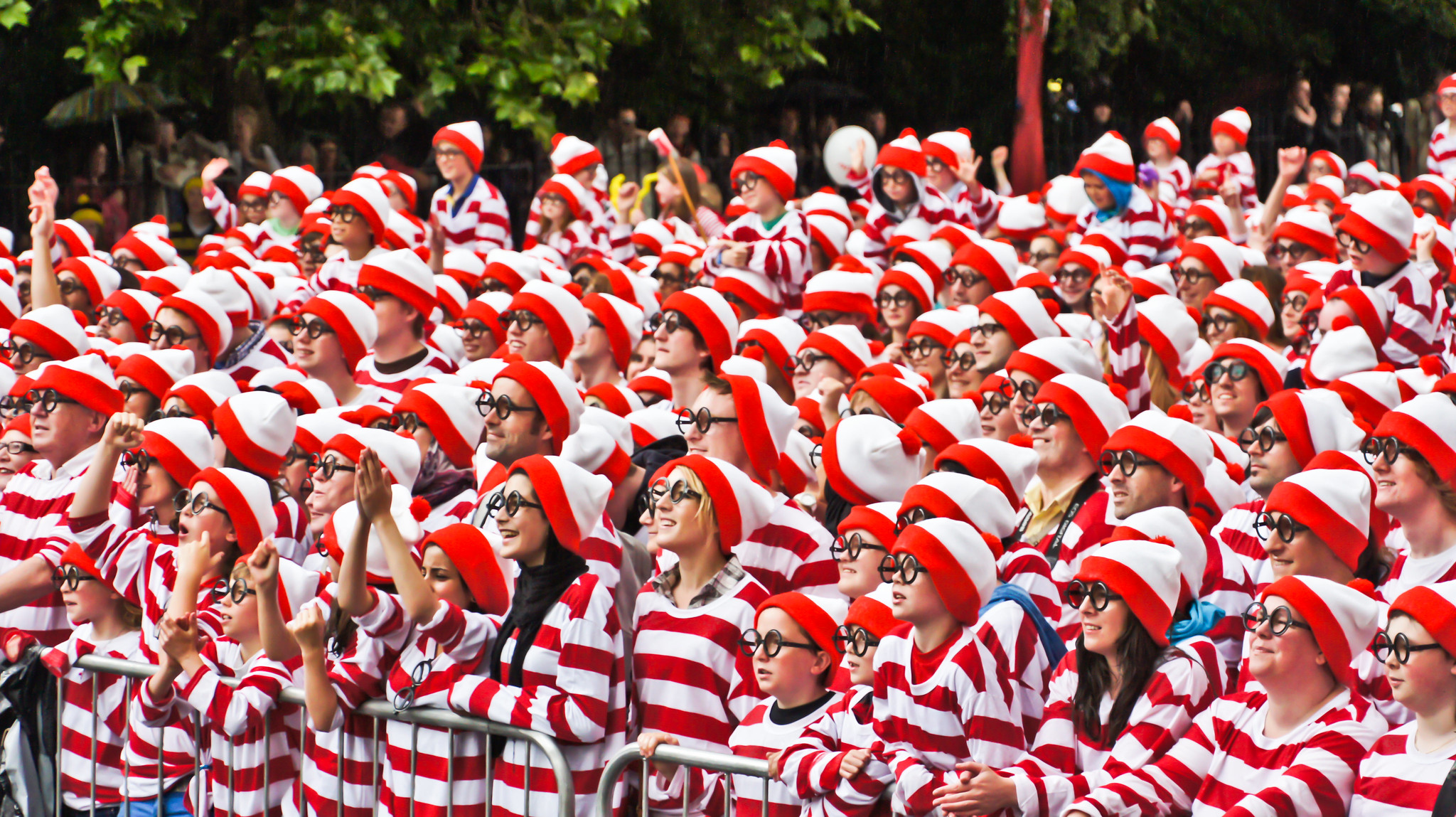
These observations suggest three requirements for a computer vision architecture:
- In the earliest layers, our network should respond similarly to the same patch, regardless of where it appears in the image: if the input is translated, the feature map produced by these layers should translate by the same amount. This property is called translation equivariance. Later in the network, global pooling or another location-agnostic readout can turn equivariant features into translation-invariant predictions.
- The earliest layers of the network should focus on local regions, without regard for the contents of the image in distant regions. This is the locality principle. Eventually, these local representations can be aggregated to make predictions at the whole image level.
- Deeper layers should combine local representations to capture progressively longer-range structure.
The distinction drawn in the first desideratum deserves precise notation. Let \(T_v\) denote the operator that translates an image by an offset \(v\), so that \([T_v \mathbf{X}]_{i,j} = [\mathbf{X}]_{i-v_1, j-v_2}\). A function \(f\) is translation equivariant if shifting its input shifts its output by the same amount, and translation invariant if shifting its input leaves the output unchanged:
\[\begin{aligned} f(T_v \mathbf{X}) &= T_v f(\mathbf{X}) && \text{(equivariance)},\\ f(T_v \mathbf{X}) &= f(\mathbf{X}) && \text{(invariance)}.\end{aligned} \tag{6.1.1}\]
On an infinite or periodically extended grid, a stride-1 convolution is equivariant. Finite boundaries, padding, and subsampling require qualifications that we develop in Section 6.3 and Section 6.5. Where we want invariance, a global aggregation in the head can supply it: such an operation discards where a feature occurred and keeps whether it occurred.
We now express these requirements mathematically.
6.1.2 Constraining the MLP
Consider an MLP whose input \(\mathbf{X}\) and immediate hidden representation \(\mathbf{H}\) are matrices of the same shape (two-dimensional tensors in code). We retain the spatial organization of both arrays.
Let \([\mathbf{X}]_{i, j}\) and \([\mathbf{H}]_{i, j}\) denote the pixel at location \((i,j)\) in the input image and hidden representation, respectively. Consequently, to have each of the hidden units receive input from each of the input pixels, we would switch from using weight matrices (as we did previously in MLPs) to representing our parameters as fourth-order weight tensors \(\mathsf{W}\). Suppose that \(\mathbf{U}\) contains biases, we could formally express the fully connected layer as
\[\begin{aligned} \left[\mathbf{H}\right]_{i, j} &= [\mathbf{U}]_{i, j} + \sum_k \sum_l[\mathsf{W}]_{i, j, k, l} [\mathbf{X}]_{k, l}\\ &= [\mathbf{U}]_{i, j} + \sum_a \sum_b [\mathsf{V}]_{i, j, a, b} [\mathbf{X}]_{i+a, j+b}.\end{aligned} \tag{6.1.2}\]
The switch from \(\mathsf{W}\) to \(\mathsf{V}\) is entirely cosmetic for now since there is a one-to-one correspondence between coefficients in both fourth-order tensors. We re-index the subscripts \((k, l)\) so that \(k = i+a\) and \(l = j+b\). In other words, we set \([\mathsf{V}]_{i, j, a, b} = [\mathsf{W}]_{i, j, i+a, j+b}\). The indices \(a\) and \(b\) run over both positive and negative offsets, covering the entire image. For any given location (\(i\), \(j\)) in the hidden representation \([\mathbf{H}]_{i, j}\), we compute its value by summing over pixels in \(x\), centered around \((i, j)\) and weighted by \([\mathsf{V}]_{i, j, a, b}\). Mapping a \(1000 \times 1000\) image (1 megapixel) to a \(1000 \times 1000\) hidden representation in this parameterization requires \(10^{12}\) parameters in a single layer. A trillion parameters is roughly a million times the number of training images we could plausibly collect for a pet classifier, so the data would not constrain most of them.
6.1.2.1 Translation Equivariance
We first impose translation equivariance (Zhang et al. 1988): shifting the input \(\mathbf{X}\) should shift the hidden representation \(\mathbf{H}\) by the same amount. For a linear map on an infinite or periodically extended grid, this requires \(\mathsf{V}\) and \(\mathbf{U}\) not to depend on \((i, j)\). As such, we have \([\mathsf{V}]_{i, j, a, b} = [\mathbf{V}]_{a, b}\) and \(\mathbf{U}\) is a constant, say \(u\). As a result, we can simplify the definition for \(\mathbf{H}\):
\[[\mathbf{H}]_{i, j} = u + \sum_a\sum_b [\mathbf{V}]_{a, b} [\mathbf{X}]_{i+a, j+b}. \tag{6.1.3}\]
This is a convolution. We are effectively weighting pixels at \((i+a, j+b)\) in the vicinity of location \((i, j)\) with coefficients \([\mathbf{V}]_{a, b}\) to obtain the value \([\mathbf{H}]_{i, j}\). \([\mathbf{V}]_{a, b}\) needs many fewer coefficients than \([\mathsf{V}]_{i, j, a, b}\) because it no longer depends on the location within the image. Consequently, the number of parameters required is no longer \(10^{12}\) but roughly \(4 \times 10^6\): there are \((2001)^2\) choices of offsets \(a, b \in \{-1000, \ldots, 1000\}\). Time-delay neural networks (TDNNs) are some of the first examples to exploit this idea (Waibel et al. 1989).
6.1.2.2 Locality
We next impose locality: computing \([\mathbf{H}]_{i, j}\) should require only a neighborhood around \((i, j)\). This means that outside some range \(|a|> \Delta\) or \(|b| > \Delta\), we should set \([\mathbf{V}]_{a, b} = 0\). Equivalently, we can rewrite \([\mathbf{H}]_{i, j}\) as
\[[\mathbf{H}]_{i, j} = u + \sum_{a = -\Delta}^{\Delta} \sum_{b = -\Delta}^{\Delta} [\mathbf{V}]_{a, b} [\mathbf{X}]_{i+a, j+b}. \tag{6.1.4}\]
This reduces the number of parameters from roughly \(4 \times 10^6\) to \((2\Delta+1)^2\), where \(\Delta\) is typically smaller than \(10\). We reduced the number of parameters by another four orders of magnitude. Equation Equation 6.1.4 defines a convolutional layer. Convolutional neural networks (CNNs) are a special family of neural networks that contain convolutional layers. In the deep learning research community, \(\mathbf{V}\) is referred to as a convolution kernel, a filter, or the layer’s learnable weights.
Where the unrestricted layer required billions of parameters, a local kernel typically requires a few hundred without altering the dimensionality of either the inputs or the hidden representations. The tradeoff for this reduction in parameters is that our features are now translation equivariant and that our layer can only incorporate local information, when determining the value of each hidden activation. All learning depends on imposing inductive bias. When that bias agrees with reality, we get sample-efficient models that generalize well to unseen data. If those biases do not agree with reality—if the same local pattern requires a different response at every location, for example— our models might struggle even to fit our training data.
Stacking convolutional layers with nonlinearities gives deeper units larger effective receptive fields, allowing them to represent larger and more complex image structure.
6.1.3 Convolutions
To understand the terminology, compare Equation 6.1.4 with the mathematical definition of convolution. In mathematics, the convolution between two functions (Rudin 1973), say \(f, g: \mathbb{R}^d \to \mathbb{R}\) is defined as
\[(f * g)(\mathbf{x}) = \int f(\mathbf{z}) g(\mathbf{x}-\mathbf{z}) d\mathbf{z}.\]
That is, we measure the overlap between \(f\) and \(g\) when one function is “flipped” and shifted by \(\mathbf{x}\). Whenever we have discrete objects, the integral turns into a sum. For instance, for vectors from the set of square-summable infinite-dimensional vectors with index running over \(\mathbb{Z}\) we obtain the following definition:
\[(f * g)(i) = \sum_a f(a) g(i-a). \tag{6.1.5}\]
For two-dimensional tensors, we have a corresponding sum with indices \((a, b)\) for \(f\) and \((i-a, j-b)\) for \(g\), respectively:
\[(f * g)(i, j) = \sum_a\sum_b f(a, b) g(i-a, j-b). \tag{6.1.6}\]
This looks similar to Equation 6.1.4, with one major difference. Rather than using \((i+a, j+b)\), we are using the difference instead. Note, though, that this distinction is mostly cosmetic since we can always match the notation between Equation 6.1.4 and Equation 6.1.6. Our original definition in Equation 6.1.4 more properly describes a cross-correlation. We will come back to this in the following section.
6.1.4 Channels
Return to the Waldo detector. The convolutional layer picks windows of a given size and weighs intensities according to the filter \(\mathsf{V}\), as demonstrated in Figure 6.1.2. We might aim to learn a model so that wherever the “waldoness” is highest, we should find a peak in the hidden layer representations.
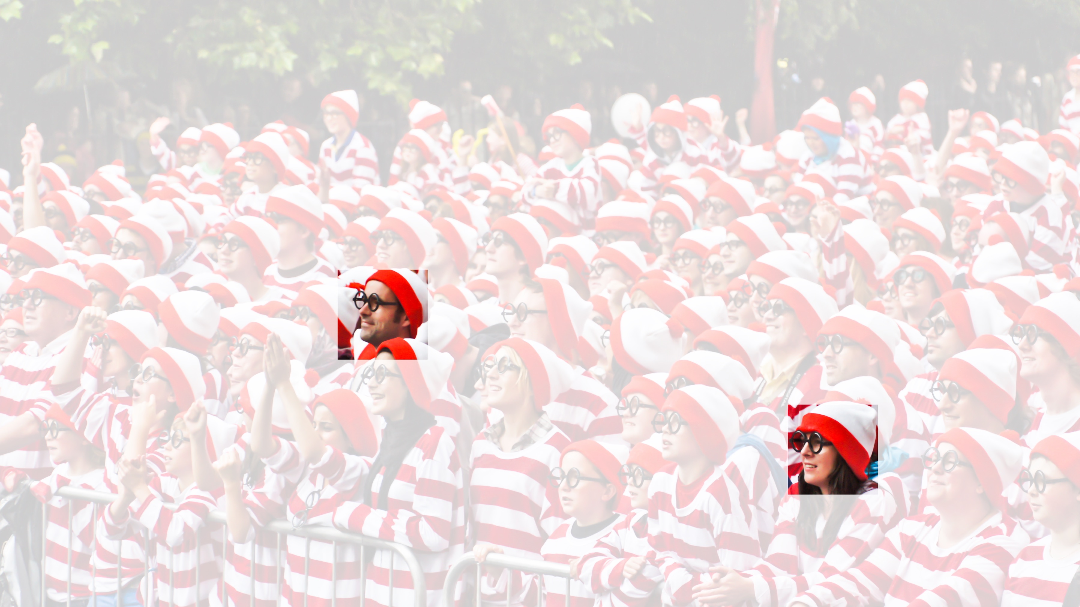
The preceding derivation omitted the three color channels in an image: red, green, and blue. In sum, images are not two-dimensional objects but rather third-order tensors, characterized by a height, width, and channel, e.g., with shape \(1024 \times 1024 \times 3\) pixels. While the first two of these axes concern spatial relationships, the third can be regarded as assigning a multidimensional representation to each pixel location. We thus index \(\mathsf{X}\) as \([\mathsf{X}]_{i, j, k}\). The convolutional filter has to adapt accordingly. Instead of \([\mathbf{V}]_{a,b}\), we now have \([\mathsf{V}]_{a,b,c}\).
We likewise formulate the hidden representation as a third-order tensor \(\mathsf{H}\), assigning a vector rather than a scalar to each spatial location. We could think of the hidden representations as comprising a number of two-dimensional grids stacked on top of each other. As in the inputs, these are sometimes called channels. They are also sometimes called feature maps, as each provides a spatialized set of learned features for the subsequent layer. In early layers, some channels may specialize in edges while others could recognize textures.
To support multiple channels in both inputs (\(\mathsf{X}\)) and hidden representations (\(\mathsf{H}\)), we can add a fourth coordinate to \(\mathsf{V}\): \([\mathsf{V}]_{a, b, c, d}\). Putting everything together we have:
\[[\mathsf{H}]_{i,j,d} = \sum_{a = -\Delta}^{\Delta} \sum_{b = -\Delta}^{\Delta} \sum_c [\mathsf{V}]_{a, b, c, d} [\mathsf{X}]_{i+a, j+b, c}, \tag{6.1.7}\]
where \(d\) indexes the output channels in the hidden representations \(\mathsf{H}\). The subsequent convolutional layer will go on to take a third-order tensor, \(\mathsf{H}\), as input. We take Equation 6.1.7, because of its generality, as the definition of a convolutional layer for multiple channels, where \(\mathsf{V}\) is a kernel or filter of the layer.
There are still many operations that we need to address. For instance, we need to figure out how to combine all the hidden representations to a single output, e.g., whether there is a Waldo anywhere in the image. We also need to decide how to compute things efficiently, how to combine multiple layers, appropriate activation functions, and how to make reasonable design choices to yield networks that are effective in practice. We turn to these issues in the remainder of the chapter.
6.1.5 Summary and Discussion
In this section we derived convolutional layers from two assumptions about low-level image processing. Translation equivariance means that the same local pattern is processed in the same way at every location; locality restricts that processing to a small neighborhood. Exact equivariance holds on an infinite or periodic grid. Boundaries, padding, and strides can break it, as the next sections will show. Some of the earliest CNN-like architectures appear in the Neocognitron (Fukushima 1982).
The parameter reduction comes from restricting the function class. It preserves a desired mapping when that mapping is local and translation equivariant, but it excludes mappings that depend on absolute position. For example, a classifier whose label changes when the same object moves from the left half of an image to the right cannot be represented by a translation- invariant head alone. The assumptions make many image problems tractable; they do not preserve arbitrary functions.
Adding channels restores some of the expressive capacity removed by locality and translation equivariance. It is natural to add channels other than red, green, and blue. Many satellite images used in agriculture and meteorology are hyperspectral, with tens to hundreds of channels that record different wavelengths. The following sections show how convolutions transform spatial dimensions and channels efficiently.
6.1.6 Exercises
- Assume that the size of the convolution kernel is \(\Delta = 0\). Show that in this case the convolution kernel implements an MLP independently for each set of channels. This leads to the Network in Network architectures (Lin et al. 2013).
- Audio data is often represented as a one-dimensional sequence.
- When might you want to impose locality and translation equivariance for audio?
- Derive the convolution operations for audio.
- Can you treat audio using the same tools as computer vision? Hint: use the spectrogram.
- Why might translation equivariance not be a good inductive bias? Give an example.
- Do you think that convolutional layers might also be applicable for text data? Which problems might you encounter with language?
- What happens with convolutions when an object is at the boundary of an image?
- Prove that the convolution is symmetric, i.e., \(f * g = g * f\).