%matplotlib inline
from d2l import torch as d2l
import math
import torch
from torch import nn9.9 Muon
The preceding optimizers treat parameters as coordinates of a vector. A network, however, contains embedding tables, hidden matrices, and normalization vectors, with most parameters in matrices. Muon uses this matrix structure to define a different preconditioned update.
The organizing idea of this chapter says an optimizer begins with a choice of descent direction, and this section makes the choice explicit: the direction of steepest descent depends on the norm used to measure the step. Under the Euclidean norm the answer is the gradient, and we recover the direction of SGD. Under the \(\ell_\infty\) norm the answer is the sign of the gradient, which resembles the limiting direction of a coordinate-normalized adaptive update but omits Adam’s moment estimates, bias correction, and \(\epsilon\). Under the spectral norm, which controls worst-case changes to a linear layer’s activations, the answer is the gradient with its singular values erased, and we arrive at Muon (Jordan et al. 2024), which since 2024 has gone from a speed-run leaderboard to trillion-parameter training runs. We derive it, implement it in about fifteen lines, compare it with AdamW on the testbeds of Section 9.6, place it in the family of preconditioned methods it belongs to, and finish by weighing the evidence.
%matplotlib inline
from d2l import jax as d2l
from flax import nnx
import jax
from jax import numpy as jnp
import math
import optax
9.9.1 The Norm Decides the Direction
9.9.1.1 Steepest Descent Under a Ball
What does it mean for a direction to be “steepest”? Linearize the loss around the current iterate, \(f(\mathbf{x} + \mathbf{d}) \approx f(\mathbf{x}) + \langle \mathbf{g}, \mathbf{d} \rangle\), and ask for the step that decreases it most among all steps of a given size:
\[ \mathbf{d}^\star = \operatorname*{argmin}_{\|\mathbf{d}\| \leq \eta} \; \langle \mathbf{g}, \mathbf{d} \rangle. \tag{9.9.1}\]
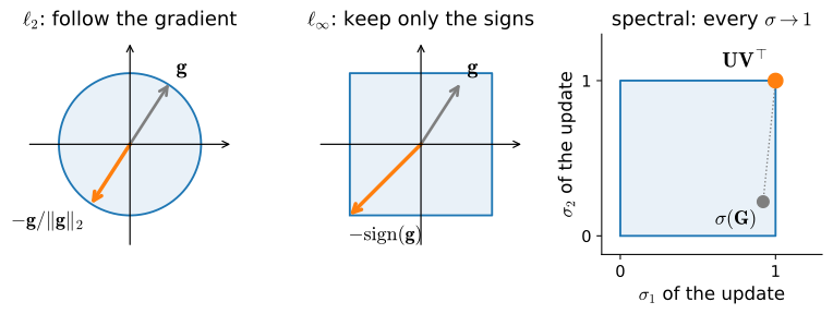
The problem is not fully posed until we say which norm defines the ball \(\|\mathbf{d}\| \leq \eta\), and different norms give genuinely different answers (Bernstein and Newhouse 2024). Under the Euclidean norm the ball is round, the minimizer points straight along \(-\mathbf{g}\), and Equation 9.9.1 returns normalized gradient descent, \(-\eta\,\mathbf{g}/\|\mathbf{g}\|_2\) — the SGD direction. Ordinary SGD takes that direction with a length that scales with \(\|\mathbf{g}\|_2\) (equivalently, it solves the regularized model \(\min_{\mathbf{d}} \langle \mathbf{g}, \mathbf{d} \rangle + \|\mathbf{d}\|_2^2 / (2\eta)\) rather than the fixed ball); each ball in this section determines the direction, while the rule for scaling the step length remains separate. Following the gradient therefore assumes Euclidean geometry, and every method in this chapter that we described as a modification of SGD can instead be read as a different answer to the same question.
Take the \(\ell_\infty\) norm, \(\|\mathbf{d}\|_\infty = \max_i |d_i|\). The ball is now a box: a step is “size \(\eta\)” as long as no single coordinate moves more than \(\eta\). To make \(\langle \mathbf{g}, \mathbf{d} \rangle\) as negative as possible we push every coordinate to its wall, and the minimizer is \(\mathbf{d}^\star = -\eta\, \mathrm{sign}(\mathbf{g})\): sign descent. This direction already appeared in Adam. In Section 9.6 we switched off Adam’s two averages (\(\beta_1 = \beta_2 = 0\), \(\epsilon \to 0\)) and were left with exactly \(\eta\,\mathrm{sign}(\mathbf{g}_t)\), and we saw that Adam’s advantage over SGD on language models tracks the advantage of sign descent (Kunstner et al. 2023). In the geometric reading, Adam is smoothed steepest descent under \(\ell_\infty\): the box moves every coordinate by the same magnitude regardless of the gradient’s coordinate scales. This is the per-coordinate equalization identified in Section 9.6, and the moment estimates are there to keep the sign stable under minibatch noise. This ball is particularly useful when coordinates have very different gradient scales, which is what the heterogeneity of language models produces.
9.9.1.2 Matrices and the Spectral Norm
Both preceding norms treat a parameter as an unstructured vector. Most parameters in the testbed instead belong to matrices: in our tiny transformer, about 95% sit in two-dimensional hidden matrices whose job is to transform activations, \(\mathbf{y} = \mathbf{W}\mathbf{x}\). For such a parameter, one useful definition of a step’s size is the largest change it can make to an activation vector. This change is governed by the spectral norm: \(\|\Delta \mathbf{W} \mathbf{x}\|_2 \leq \|\Delta \mathbf{W}\|_2\, \|\mathbf{x}\|_2\), with equality for the worst-case input. The spectral norm \(\|\Delta \mathbf{W}\|_2\) is the largest singular value, and hence the largest factor by which the update can stretch any activation vector passing through the layer. Flattening the matrix and using the Euclidean norm of the entries (the Frobenius norm) instead adds up energy across all \(\min(m, n)\) singular directions, so it can call an update “large” even when its effect on every activation is small; controlling the spectral norm of updates is also required to preserve feature learning when scaling the network (Yang et al. 2023), a thread Section 9.11 picks up.
So let the ball be spectral and solve Equation 9.9.1 for a matrix parameter with gradient \(\mathbf{G}\). Write the reduced singular value decomposition \(\mathbf{G} = \mathbf{U} \boldsymbol{\Sigma} \mathbf{V}^\top\). The steepest step is the orthogonalized gradient:
\[ \Delta \mathbf{W}^\star = \operatorname*{argmin}_{\|\Delta \mathbf{W}\|_2 \leq \eta} \; \langle \mathbf{G}, \Delta \mathbf{W} \rangle = -\eta\, \mathbf{U} \mathbf{V}^\top. \tag{9.9.2}\]
The argument is one line of duality. For any \(\mathbf{A}\) with \(\|\mathbf{A}\|_2 \leq 1\) we have \(\langle \mathbf{G}, \mathbf{A} \rangle = \mathrm{tr}(\boldsymbol{\Sigma}\, \mathbf{U}^\top \mathbf{A} \mathbf{V}) = \sum_i \sigma_i\, (\mathbf{U}^\top \mathbf{A} \mathbf{V})_{ii} \leq \sum_i \sigma_i\), since no entry of a matrix with unit spectral norm exceeds one; choosing \(\mathbf{A} = \mathbf{U}\mathbf{V}^\top\) attains the bound, and negating it attains the minimum. (Checking the diagonal-entry claim is an exercise; the surrounding theory, including what this has to do with preconditioning, lives in Section 26.2.6.)
Equation Equation 9.9.2 equalizes singular directions. The gradient \(\mathbf{U}\boldsymbol{\Sigma}\mathbf{V}^\top\) names a set of directions and weights them by singular values that, for real training gradients, are dominated by a few large ones. The steepest spectral step keeps the singular vectors and replaces every nonzero singular value by one: every direction the gradient identifies moves at the same rate. This is per-direction equalization, in whatever basis the gradient supplies, whereas Adam manages only per-coordinate equalization in the axis basis it is handed. The reasoning also says where it does not apply. An embedding table never multiplies a dense activation vector; its input is one-hot, each row is looked up in isolation, and the norm the input induces is the largest row norm rather than the spectral norm — a geometry for which spectral orthogonalization is an inappropriate geometry (Bernstein 2025). Embeddings, the output head, and the one-dimensional vectors stay with AdamW, and the parameter-group split becomes an optimizer assignment. Table 9.9.1 summarizes the three geometries.
:Steepest descent under three norms. Each ball yields a closed-form step and suits a different population of the parameter census.
| ball on the step | steepest step | natural habitat |
|---|---|---|
| Euclidean, \(\|\mathbf{d}\|_2 \leq \eta\) | \(-\eta\, \mathbf{g} / \|\mathbf{g}\|_2\) | no structure assumed (SGD direction) |
| box, \(\|\mathbf{d}\|_\infty \leq \eta\) | \(-\eta\, \mathrm{sign}(\mathbf{g})\) | coordinates of very different scale (Adam family) |
| spectral, \(\|\Delta \mathbf{W}\|_2 \leq \eta\) | \(-\eta\, \mathbf{U}\mathbf{V}^\top\) | hidden matrices acting on activations (Muon) |
Figure 9.9.1 draws the three choices for one gradient.
9.9.2 Orthogonalization by Newton–Schulz
Equation Equation 9.9.2 asks for \(\mathbf{U}\mathbf{V}^\top\), and computing an SVD for every matrix at every step is out of the question: SVD is expensive, hard to parallelize well on accelerators, and unavailable in the low-precision arithmetic that training runs in. Muon uses a classical matrix iteration for this computation. For any odd polynomial applied as a matrix polynomial,
\[ p(\mathbf{X}) = a\mathbf{X} + b\,(\mathbf{X}\mathbf{X}^\top)\mathbf{X} + c\,(\mathbf{X}\mathbf{X}^\top)^2\mathbf{X} = \mathbf{U}\, p(\boldsymbol{\Sigma})\, \mathbf{V}^\top, \tag{9.9.3}\]
because each factor of \(\mathbf{X}\mathbf{X}^\top\) contributes \(\mathbf{U}\boldsymbol{\Sigma}^2\mathbf{U}^\top\) and the orthogonal factors telescope. A polynomial in the matrix is the same polynomial applied to each singular value, with \(\mathbf{U}\) and \(\mathbf{V}\) untouched. So we can drive all nonzero singular values toward \(1\), never computing them, by iterating a scalar polynomial that has \(1\) as an attracting fixed point on \((0, 1]\). Dividing \(\mathbf{X}\) by its Frobenius norm first guarantees every nonzero singular value starts in \((0, 1]\); exact zeros are fixed points of any odd polynomial, so a rank-deficient matrix stays rank-deficient.
The classical Newton–Schulz cubic does this with \(p(x) = \tfrac{3}{2}x - \tfrac{1}{2}x^3\), but its progress near zero is slow: a tiny singular value only grows by a factor of \(1.5\) per iteration. Jordan et al. (2024) instead tuned the quintic
\[ p(x) = 3.4445\,x - 4.7750\,x^3 + 2.0315\,x^5, \tag{9.9.4}\]
whose slope at the origin is \(3.4445\), so a direction hundreds of times weaker than the dominant one still reaches order \(1\) within five iterations. The limitation of the aggressive slope is that the iteration does not converge to \(1\); it oscillates in a band around it. For an optimizer this is a fine trade: we need “all directions move at roughly the same rate”, not machine-precision orthogonality, and the iteration is stable enough to run in bfloat16. Five iterations of Equation 9.9.4 is a handful of matrix multiplications, the operation GPUs are best at; the implementation transposes a tall matrix first, so the Gram factor \(\mathbf{X}\mathbf{X}^\top\) is the smaller of the two squares.
def newton_schulz(M, num_iters=5, eps=1e-7):
    a, b, c = 3.4445, -4.7750, 2.0315
    tall = M.shape[0] > M.shape[1]
    X = M.T if tall else M  # keep the Gram factor X @ X.T small
    X = X / (X.norm() + eps)
    for _ in range(num_iters):
        A = X @ X.T
        X = a * X + (b * A + c * A @ A) @ X
    return X.T if tall else X
def newton_schulz(M, num_iters=5, eps=1e-7):
a, b, c = 3.4445, -4.7750, 2.0315
tall = M.shape[0] > M.shape[1]
X = M.T if tall else M # keep the Gram factor X @ X.T small
X = X / (jnp.linalg.norm(X) + eps)
for _ in range(num_iters):
A = X @ X.T
X = a * X + (b * A + c * A @ A) @ X
return X.T if tall else XThe following experiment measures the iteration. We take a random \(96 \times 64\) matrix, whose singular values after normalization span an order of magnitude, and plot the spectrum after 0, 1, 3, and 5 iterations. (The SVD below is for measuring the result; the iteration itself never computes one.)
torch.manual_seed(0)
G = torch.randn(96, 64)
sigmas = [torch.linalg.svdvals(newton_schulz(G, num_iters=k))
          for k in (0, 1, 3, 5)]
d2l.plot(torch.arange(1, 65), sigmas, 'index', 'singular value',
         legend=[f'k = {k}' for k in (0, 1, 3, 5)], yscale='log')
print(f'singular values after 5 iterations: '
      f'[{sigmas[-1].min():.2f}, {sigmas[-1].max():.2f}]')
singular values after 5 iterations: [0.68, 1.13]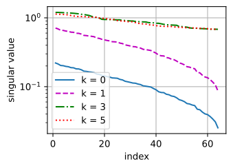
G = jax.random.normal(jax.random.key(0), (96, 64))
sigmas = [jnp.linalg.svd(newton_schulz(G, num_iters=k), compute_uv=False)
          for k in (0, 1, 3, 5)]
d2l.plot(jnp.arange(1, 65), sigmas, 'index', 'singular value',
         legend=[f'k = {k}' for k in (0, 1, 3, 5)], yscale='log')
print(f'singular values after 5 iterations: '
      f'[{sigmas[-1].min():.2f}, {sigmas[-1].max():.2f}]')
singular values after 5 iterations: [0.68, 1.13]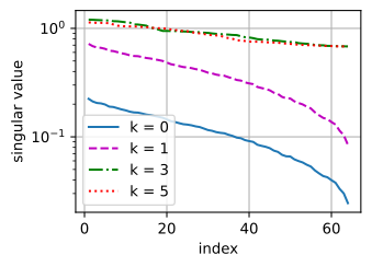
One iteration lifts the whole spectrum; three compress it to within a factor of a few; after five, every singular value sits in a band around \(1\), from roughly \(0.7\) to \(1.2\). That is \(\mathbf{U}\mathbf{V}^\top\) for an optimizer’s purposes, at the cost of fifteen matrix multiplications. (A nearly singular direction takes a few more iterations to climb out, at \(3.4\)-fold per pass; the exercises probe how much that matters in training.)
9.9.3 Muon from Scratch
9.9.3.1 The Update
Muon combines momentum, Nesterov look-ahead, and approximate orthogonalization. Gradients are noisy, so we do not orthogonalize the raw gradient. We keep a momentum buffer, the leaky average of Section 9.5, with the same \(\mu = 0.95\) used by its authors, and we hand Newton–Schulz the Nesterov blend \(\mathbf{G}_t + \mu \mathbf{M}_t\): the gradient plus a look ahead along the freshly updated buffer. The result is then rescaled once per matrix shape:
\[ \mathbf{M}_t = \mu\, \mathbf{M}_{t-1} + \mathbf{G}_t, \qquad \mathbf{W}_{t+1} = \mathbf{W}_t - \eta \cdot 0.2 \sqrt{\max(m, n)}\; \mathrm{NS}_5(\mathbf{G}_t + \mu\, \mathbf{M}_t) \tag{9.9.5}\]
for an \(m \times n\) matrix. The scale factor deserves a sentence, because it is what makes Muon a drop-in teammate for AdamW. An orthogonalized matrix has \(\min(m, n)\) singular values equal to \(1\), hence Frobenius norm \(\sqrt{\min(m, n)}\) and root-mean-square entry size \(1 / \sqrt{\max(m, n)}\): without correction, wide matrices would take smaller per-entry steps than square ones. Multiplying by \(0.2\sqrt{\max(m, n)}\) makes every matrix’s update have entrywise RMS \(0.2\,\eta\) regardless of shape, which matches the typical RMS of an AdamW update. With this convention, introduced for the Moonlight model, a learning rate and weight decay tuned for AdamW transfer directly to Muon (Liu et al. 2025), so the hybrid optimizer below needs only one learning rate. (The original Muon used a different shape factor, and the theoretically derived scale is \(\sqrt{\text{fan-out} / \text{fan-in}}\) per Bernstein (2025); the distinction matters when transferring across model widths, which is Section 9.11’s subject.)
The implementation is short. reshape handles the one wrinkle we will need later: a convolution kernel is a matrix in disguise, so flattening it lets the same code precondition CNNs. (It has one row per output channel in PyTorch’s OIHW layout and one column in Flax’s HWIO; the two are transposes of each other, and orthogonalization commutes with transposition.) On our tiny matrices the fifteen extra multiplications add a visible fraction to the step time; at production scale, where the forward and backward passes dwarf them, the reported overhead is around one percent of the training FLOPs (Jordan et al. 2024).
class Muon(torch.optim.Optimizer):
    """Steepest descent under the spectral norm: orthogonalized momentum."""
    def __init__(self, params, lr, momentum=0.95):
        super().__init__(params, dict(lr=lr, momentum=momentum))

    @torch.no_grad()
    def step(self):
        for group in self.param_groups:
            for p in group['params']:
                buf = self.state[p].setdefault('buf', torch.zeros_like(p))
                buf.mul_(group['momentum']).add_(p.grad)
                G = p.grad + group['momentum'] * buf  # Nesterov momentum
                M = G.reshape(len(G), -1)             # flattens conv kernels
                O = newton_schulz(M).reshape(p.shape)
                p.add_(O, alpha=-group['lr'] * 0.2 * math.sqrt(max(M.shape)))
def scratch_muon(learning_rate, momentum=0.95):
def init(params):
return jax.tree.map(jnp.zeros_like, params)
def update(grads, bufs, params=None):
bufs = jax.tree.map(lambda b, g: momentum * b + g, bufs, grads)
def step(g, b):
G = g + momentum * b # Nesterov momentum
M = G.reshape(-1, G.shape[-1]) # flattens conv kernels
O = newton_schulz(M).reshape(G.shape)
return -learning_rate * 0.2 * math.sqrt(max(M.shape)) * O
return jax.tree.map(step, grads, bufs), bufs
return optax.GradientTransformation(init, update)9.9.3.2 Dividing the Census
Muon is an optimizer for hidden matrices only, so a real training run is a hybrid: the parameter-group mechanism of Section 9.7, with the census deciding who goes where. Hidden matrices go to Muon; embeddings, the output head, and every one-dimensional tensor go to AdamW.
data = d2l.TimeMachine(batch_size=64, num_steps=64, tokenization='char',
                       num_train=100000)

def split_lm(model):
    hidden, rest = [], []
    for name, p in model.named_parameters():
        is_hidden = p.ndim == 2 and 'emb' not in name and 'head' not in name
        (hidden if is_hidden else rest).append(p)
    return hidden, rest

model = d2l.TinyLM(len(data.vocab))
hidden, rest = split_lm(model)
print(f'Muon:  {len(hidden):>2} tensors, '
      f'{sum(p.numel() for p in hidden):>7} parameters')
print(f'AdamW: {len(rest):>2} tensors, '
      f'{sum(p.numel() for p in rest):>7} parameters')
Muon: 8 tensors, 393216 parameters
AdamW: 22 tensors, 18972 parametersdata = d2l.TimeMachine(batch_size=64, num_steps=64, tokenization='char',
num_train=100000)
model = d2l.TinyLM(len(data.vocab))
counts = {'muon': [0, 0], 'adamw': [0, 0]}
for path, p in nnx.to_flat_state(nnx.state(model, nnx.Param)):
name = '.'.join(str(k) for k in path)
is_hidden = p.ndim == 2 and 'emb' not in name and 'head' not in name
group = counts['muon' if is_hidden else 'adamw']
group[0] += 1
group[1] += p.size
for name, (num, size) in counts.items():
print(f'{name}: {num:>2} tensors, {size:>7} parameters')muon: 8 tensors, 393216 parameters
adamw: 22 tensors, 18972 parametersThe eight hidden matrices hold about 95% of the parameters. Note what the split does to optimizer state: AdamW carries two buffers per parameter, Muon one, so the hybrid’s state memory is nearly half of all-AdamW’s, an as follows from the state-memory accounting in Section 9.7. The factory below builds the hybrid; with the RMS-matched scale of 1, both halves share a single learning rate.
class MultiOptimizer:
    """Apply independent optimizers to disjoint parameter groups."""
    def __init__(self, *optimizers):
        self.optimizers = optimizers

    def step(self):
        for opt in self.optimizers:
            opt.step()

    def zero_grad(self):
        for opt in self.optimizers:
            opt.zero_grad()

def muon_adamw(hidden, rest, lr):
    return MultiOptimizer(Muon(hidden, lr=lr),
                          torch.optim.AdamW(rest, lr=lr, weight_decay=0.0))
def muon_adamw(lr, exclude=('emb', 'head')):
def labels(params):
def label(path, p):
name = jax.tree_util.keystr(path)
is_hidden = (p.ndim >= 2
and not any(s in name for s in exclude))
return 'muon' if is_hidden else 'adamw'
return jax.tree_util.tree_map_with_path(label, params)
return optax.multi_transform(
{'muon': scratch_muon(lr),
'adamw': optax.adamw(lr, weight_decay=0.0)}, labels)9.9.3.3 Comparison on the Language Model
The protocol is the one from Section 9.6: same model, same initialization, 2,000 steps at a constant learning rate, a four-point learning-rate grid per contestant, best final training loss speaks for its family. “Tuned” in what follows means the best of this coarse four-point grid, nothing finer. Weight decay is switched off in both arms so that the only difference between them is the direction of the update on the hidden matrices. First the baseline, all parameters on AdamW:
def final_loss(losses, k=100):
    v = sum(losses[-k:]) / k
    return v if math.isfinite(v) else float('inf')

def smooth(losses, k=25):
    return [sum(losses[i:i + k]) / k
            for i in range(0, len(losses) - k + 1, k)]

def run_lm(make_optimizer, lrs, num_steps=2000):
    curves = {}
    for lr in lrs:
        torch.manual_seed(0)
        model = d2l.TinyLM(len(data.vocab))
        curves[lr] = d2l.train_lm(model, data, make_optimizer(model, lr),
                                  num_steps)
        print(f'lr {lr:g}: final loss {final_loss(curves[lr]):.3f}')
    return curves

adamw_lm = run_lm(
    lambda model, lr: torch.optim.AdamW(model.parameters(), lr,
                                        weight_decay=0.0),
    lrs=[3e-4, 1e-3, 3e-3, 1e-2])
lr 0.0003: final loss 1.506
lr 0.001: final loss 1.157
lr 0.003: final loss 0.913
lr 0.01: final loss 0.960def final_loss(losses, k=100):
v = sum(losses[-k:]) / k
return v if math.isfinite(v) else float('inf')
def smooth(losses, k=25):
return [sum(losses[i:i + k]) / k
for i in range(0, len(losses) - k + 1, k)]
def run_lm(make_tx, lrs, num_steps=2000):
curves = {}
for lr in lrs:
model = d2l.TinyLM(len(data.vocab), rngs=nnx.Rngs(0))
optimizer = nnx.Optimizer(model, make_tx(lr), wrt=nnx.Param)
curves[lr] = d2l.train_lm(model, data, optimizer, num_steps)
print(f'lr {lr:g}: final loss {final_loss(curves[lr]):.3f}')
return curves
adamw_lm = run_lm(lambda lr: optax.adamw(lr, weight_decay=0.0),
lrs=[3e-4, 1e-3, 3e-3, 1e-2])lr 0.0003: final loss 1.310
lr 0.001: final loss 1.025
lr 0.003: final loss 1.022
lr 0.01: final loss 2.287We evaluate the hybrid over the same grid. RMS matching makes the nominal rates comparable between the two optimizers:
muon_lm = run_lm(
    lambda model, lr: muon_adamw(*split_lm(model), lr),
    lrs=[3e-4, 1e-3, 3e-3, 1e-2])
lr 0.0003: final loss 1.519
lr 0.001: final loss 1.074
lr 0.003: final loss 0.928
lr 0.01: final loss 0.827muon_lm = run_lm(muon_adamw, lrs=[3e-4, 1e-3, 3e-3, 1e-2])lr 0.0003: final loss 1.243
lr 0.001: final loss 0.684
lr 0.003: final loss 0.616
lr 0.01: final loss 0.907best_adamw = min(adamw_lm, key=lambda lr: final_loss(adamw_lm[lr]))
best_muon = min(muon_lm, key=lambda lr: final_loss(muon_lm[lr]))
d2l.plot(list(range(0, 2000, 25)),
[smooth(adamw_lm[best_adamw]), smooth(muon_lm[best_muon])],
'step', 'training loss',
legend=[f'AdamW, lr {best_adamw:g}',
f'Muon + AdamW, lr {best_muon:g}'])
print(f'final perplexity: '
f'AdamW {math.exp(final_loss(adamw_lm[best_adamw])):.2f}, '
f'Muon+AdamW {math.exp(final_loss(muon_lm[best_muon])):.2f}')final perplexity: AdamW 2.49, Muon+AdamW 2.29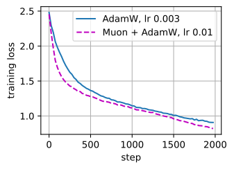
final perplexity: AdamW 2.78, Muon+AdamW 1.85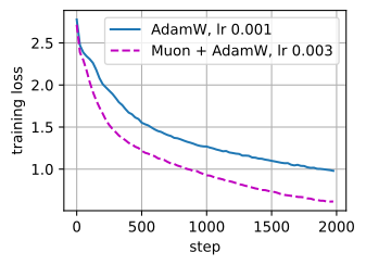
After tuning both methods, the hybrid finishes a few percent lower in perplexity than AdamW. This single-seed result supports only a modest difference, although the hybrid also uses nearly half the optimizer state. A 0.4M-parameter model trained for a minute cannot establish a broader ranking. The fair-tuning literature discussed at the end of this section measures Muon-family gains in tens of percent of data efficiency at small scale, an effect two thousand steps can only hint at. The experiment demonstrates the mechanism rather than providing a benchmark; before drawing conclusions, consider the same comparison in the JAX tab, where the identical protocol produces a very different margin.
In the JAX run, the tuned hybrid finishes several tenths of a nat below tuned AdamW and remains lower throughout training. This margin does not support a general conclusion: the PyTorch tab runs the identical protocol and ends with a far smaller edge. The two frameworks differ in details as mundane as default layer initialization, and comparisons this small are sensitive to all of them. Across both tabs, the supported conclusion is narrower: the hybrid finished below AdamW in both single-seed runs, narrowly in PyTorch and by a wider margin in JAX, while using nearly half the optimizer state. The differing margins show that small optimizer comparisons are protocol-sensitive, and the fair-tuning studies at the end of the section exist precisely because of it. The demo is mechanism, not benchmark.
9.9.3.4 Comparison on a CNN
Section 9.6 found that Adam’s substantial advantage over SGD on the language model nearly vanished on a CNN. We apply the same comparison to Muon. We reuse the compact Fashion-MNIST CNN from that section, along with its test-accuracy check; reshape in the update flattens each convolution kernel to a matrix (one row per output channel in PyTorch, one column in Flax), and the output head stays with AdamW.
fashion = d2l.FashionMNIST(batch_size=256)

def make_cnn():
    return nn.Sequential(
        nn.LazyConv2d(32, kernel_size=3, padding=1), nn.ReLU(),
        nn.MaxPool2d(2),
        nn.LazyConv2d(64, kernel_size=3, padding=1), nn.ReLU(),
        nn.MaxPool2d(2),
        nn.Flatten(), nn.LazyLinear(128), nn.ReLU(), nn.LazyLinear(10))

def split_cnn(model):
    head = model[-1].weight
    hidden = [p for p in model.parameters()
              if p.ndim >= 2 and p is not head]
    rest = [p for p in model.parameters() if p.ndim < 2 or p is head]
    return hidden, rest

def test_accuracy(model, data):
    device = d2l.try_gpu()
    model.eval()
    correct = total = 0
    with torch.no_grad():
        for X, y in data.val_dataloader():
            X, y = X.to(device), y.to(device)
            correct += float((model(X).argmax(axis=1) == y).sum())
            total += y.numel()
    return correct / total

def run_cnn(make_optimizer, lrs, num_steps=2000):
    curves, accs = {}, {}
    for lr in lrs:
        torch.manual_seed(0)
        model = make_cnn()
        model(next(iter(fashion.train_dataloader()))[0])
        curves[lr] = d2l.train_lm(model, fashion, make_optimizer(model, lr),
                                  num_steps)
        accs[lr] = test_accuracy(model, fashion)
        print(f'lr {lr:g}: final loss {final_loss(curves[lr]):.3f}, '
              f'test accuracy {accs[lr]:.3f}')
    return curves, accs

adamw_cnn, adamw_acc = run_cnn(
    lambda model, lr: torch.optim.AdamW(model.parameters(), lr,
                                        weight_decay=0.0),
    lrs=[3e-4, 1e-3, 3e-3, 1e-2])
lr 0.0003: final loss 0.284, test accuracy 0.889
lr 0.001: final loss 0.192, test accuracy 0.915
lr 0.003: final loss 0.110, test accuracy 0.916
lr 0.01: final loss 0.169, test accuracy 0.897fashion = d2l.FashionMNIST(batch_size=256)
class FashionCNN(nnx.Module):
def __init__(self, rngs=None):
rngs = nnx.Rngs(0) if rngs is None else rngs
self.conv1 = nnx.Conv(1, 32, kernel_size=(3, 3), rngs=rngs)
self.conv2 = nnx.Conv(32, 64, kernel_size=(3, 3), rngs=rngs)
self.fc1 = nnx.Linear(64 * 7 * 7, 128, rngs=rngs)
self.fc2 = nnx.Linear(128, 10, rngs=rngs)
def __call__(self, X):
X = nnx.max_pool(nnx.relu(self.conv1(X)), window_shape=(2, 2),
strides=(2, 2))
X = nnx.max_pool(nnx.relu(self.conv2(X)), window_shape=(2, 2),
strides=(2, 2))
X = X.reshape(X.shape[0], -1)
return self.fc2(nnx.relu(self.fc1(X)))
def test_accuracy(model, data):
correct = total = 0
for X, y in data.val_dataloader():
pred = model(jnp.asarray(X)).argmax(axis=1)
correct += float((pred == jnp.asarray(y)).sum())
total += y.shape[0]
return correct / total
def run_cnn(make_tx, lrs, num_steps=2000):
curves, accs = {}, {}
for lr in lrs:
model = FashionCNN(rngs=nnx.Rngs(0))
optimizer = nnx.Optimizer(model, make_tx(lr), wrt=nnx.Param)
curves[lr] = d2l.train_lm(model, fashion, optimizer, num_steps)
accs[lr] = test_accuracy(model, fashion)
print(f'lr {lr:g}: final loss {final_loss(curves[lr]):.3f}, '
f'test accuracy {accs[lr]:.3f}')
return curves, accs
adamw_cnn, adamw_acc = run_cnn(lambda lr: optax.adamw(lr, weight_decay=0.0),
lrs=[3e-4, 1e-3, 3e-3, 1e-2])lr 0.0003: final loss 0.230, test accuracy 0.893
lr 0.001: final loss 0.155, test accuracy 0.916
lr 0.003: final loss 0.103, test accuracy 0.920
lr 0.01: final loss 0.136, test accuracy 0.906muon_cnn, muon_acc = run_cnn(
lambda model, lr: muon_adamw(*split_cnn(model), lr),
lrs=[3e-4, 1e-3, 3e-3, 1e-2])lr 0.0003: final loss 0.164, test accuracy 0.912
lr 0.001: final loss 0.031, test accuracy 0.921
lr 0.003: final loss 0.025, test accuracy 0.914
lr 0.01: final loss 0.102, test accuracy 0.903muon_cnn, muon_acc = run_cnn(lambda lr: muon_adamw(lr, exclude=('fc2',)),
lrs=[3e-4, 1e-3, 3e-3, 1e-2])lr 0.0003: final loss 0.126, test accuracy 0.915
lr 0.001: final loss 0.026, test accuracy 0.919
lr 0.003: final loss 0.026, test accuracy 0.915
lr 0.01: final loss 0.105, test accuracy 0.908best_adamw_cnn = min(adamw_cnn, key=lambda lr: final_loss(adamw_cnn[lr]))
best_muon_cnn = min(muon_cnn, key=lambda lr: final_loss(muon_cnn[lr]))
d2l.plot(list(range(0, 2000, 25)),
[smooth(adamw_cnn[best_adamw_cnn]), smooth(muon_cnn[best_muon_cnn])],
'step', 'training loss',
legend=[f'AdamW, lr {best_adamw_cnn:g}',
f'Muon + AdamW, lr {best_muon_cnn:g}'])
print(f'test accuracy: AdamW {adamw_acc[best_adamw_cnn]:.3f}, '
f'Muon+AdamW {muon_acc[best_muon_cnn]:.3f}')test accuracy: AdamW 0.916, Muon+AdamW 0.914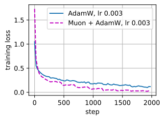
test accuracy: AdamW 0.920, Muon+AdamW 0.915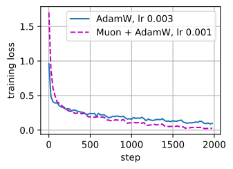
The two metrics give different conclusions. On training loss the hybrid reaches lower values: orthogonalized updates drive this small CNN into its memorization regime several times faster. On test accuracy, the deployment metric in this experiment, the two land within about a point of each other. Optimizing faster and predicting better are different claims, and on a small, quickly saturated task the second changes little. This resembles the small difference that Section 9.6 found between Adam and SGD here. The same conclusion applies: an optimizer comparison is a statement about a workload and a metric, not a universal ranking.
9.9.3.5 Library Implementations
PyTorch ships Muon in core since version 2.9. Mirroring our scratch version, torch.optim.Muon accepts only the 2-D hidden matrices (its documentation directs embeddings, biases, and heads to AdamW), applies Nesterov-style momentum before orthogonalizing, and offers the RMS-matched scale of 1 as adjust_lr_fn='match_rms_adamw'. Its default weight decay is 0.1, not zero, so we switch it off to match the protocol above.
Optax ships Muon in optax.contrib. Unlike our scratch version it manages the split internally: parameters marked with MuonDimensionNumbers are orthogonalized, while all other parameters use Adam. By default every 2-D parameter is treated as a hidden matrix, which would orthogonalize the embedding tables too, so we pass an explicit spec that sends embeddings and the head to Adam; consistent_rms=0.2 selects the RMS-matched scale of 1.
torch.manual_seed(0)
model = d2l.TinyLM(len(data.vocab))
hidden, rest = split_lm(model)
optimizer = MultiOptimizer(
    torch.optim.Muon(hidden, lr=best_muon, momentum=0.95, nesterov=True,
                     weight_decay=0.0, adjust_lr_fn='match_rms_adamw'),
    torch.optim.AdamW(rest, lr=best_muon, weight_decay=0.0))
losses = d2l.train_lm(model, data, optimizer, 2000)
print(f'final loss {final_loss(losses):.3f}')
final loss 0.840def muon_spec(params):
def spec(path, p):
name = jax.tree_util.keystr(path)
if p.ndim == 2 and 'emb' not in name and 'head' not in name:
return optax.contrib.MuonDimensionNumbers()
return None
return jax.tree_util.tree_map_with_path(spec, params)
model = d2l.TinyLM(len(data.vocab), rngs=nnx.Rngs(0))
tx = optax.contrib.muon(learning_rate=best_muon, consistent_rms=0.2,
beta=0.95, nesterov=True, weight_decay=0.0,
muon_weight_dimension_numbers=muon_spec)
optimizer = nnx.Optimizer(model, tx, wrt=nnx.Param)
losses = d2l.train_lm(model, data, optimizer, 2000)
print(f'final loss {final_loss(losses):.3f}')final loss 0.5729.9.4 The Preconditioning Family
Muon is closely related to other preconditioning methods. It can be viewed to be the frugal child of a long line. Every branch answers the question posed in Section 9.2: gradient descent assumes round level sets, real losses have curved ones, and some matrix should reshape the gradient accordingly. Adam estimates a diagonal such matrix from gradient history. The methods below estimate structure per layer, exploiting the same fact Muon does: parameters come in matrices.
K-FAC (Martens and Grosse 2015) is the family’s ancestor. The Fisher information matrix measures curvature between the distributions the model defines, and K-FAC approximates each layer’s block of it as a Kronecker product of two small matrices: the second moments of the layer’s inputs and of its output gradients. Preconditioning by a Kronecker product costs two small inverses rather than one enormous one, which made second-order-style updates feasible for neural networks and connected them to the natural gradient of Amari (1998) .
Shampoo (Gupta et al. 2018) keeps the two-sided structure but builds the factors the AdaGrad way, from accumulated gradient statistics, preconditioning each gradient matrix as \(\mathbf{L}_t^{-1/4} \mathbf{G}_t \mathbf{R}_t^{-1/4}\) with \(\mathbf{L}_t = \sum_s \mathbf{G}_s \mathbf{G}_s^\top\) and \(\mathbf{R}_t = \sum_s \mathbf{G}_s^\top \mathbf{G}_s\). A distributed implementation of Shampoo won the external-tuning track of the AlgoPerf benchmark, finishing its workloads about 30% faster than the tuned AdamW baseline (Dahl et al. 2023; Kasimbeg et al. 2025) — strong protocol-controlled evidence for matrix preconditioning. SOAP (Vyas et al. 2024) refines it further by running Adam inside Shampoo’s slowly refreshed eigenbasis, cutting the overhead between factor recomputations.
Muon has the following relationship to Shampoo: it is Shampoo with the memory removed. Switch off Shampoo’s accumulators, keeping only the current gradient with SVD \(\mathbf{G} = \mathbf{U}\boldsymbol{\Sigma}\mathbf{V}^\top\), and
\[ (\mathbf{G}\mathbf{G}^\top)^{-1/4}\, \mathbf{G}\, (\mathbf{G}^\top\mathbf{G})^{-1/4} = \mathbf{U}\boldsymbol{\Sigma}^{-1/2}\mathbf{U}^\top \cdot \mathbf{U}\boldsymbol{\Sigma}\mathbf{V}^\top \cdot \mathbf{V}\boldsymbol{\Sigma}^{-1/2}\mathbf{V}^\top = \mathbf{U}\mathbf{V}^\top, \tag{9.9.6}\]
the orthogonalized gradient again (Bernstein and Newhouse 2024). What Muon discards is the preconditioner state and the factor inverses; what it keeps is the geometry. On the other side of the tree, the same anatomy identifies Lion (Chen et al. 2023) as the lean member of the sign branch: an update found by symbolic program search, one momentum buffer and a sign, steepest descent under \(\ell_\infty\) with even less state than Adam. You will implement it in the exercises in about six lines. Section 26.2.6 assembles the full ladder with the derivations, from diagonal through Kronecker to spectral.
9.9.5 Large-Scale Use of Muon
Muon’s rise was unusually public. It debuted in late 2024 not in a paper but as a record on the NanoGPT speedrun (Jordan and contributors 2024), a standing competition to train a fixed GPT-2-class model to a fixed validation loss on fixed hardware in the least wall-clock time. The speedrun provides a transparent experimental record: one variable changes per record, the diff is public, and anyone can rerun it. Its headline number mixes optimizer, architecture, and data-schedule improvements, so it should not be read as an optimizer benchmark: a baseline of 45 minutes came down to a few minutes in under two years. Individual records do isolate single changes, though, and Muon’s debut cut the then-record by roughly a third.
Production adoption followed within months. Moonshot’s Moonlight report demonstrated Muon at multi-billion-parameter scale, introduced the RMS-matching convention of 1, and reported matched losses for roughly half the training compute of its AdamW baseline (Liu et al. 2025). Kimi K2, a trillion-parameter mixture-of-experts model, was pretrained on 15.5 trillion tokens with MuonClip: Muon plus a cap on attention logits (QK-clip) to contain the instability that surfaced at that scale. It reports zero loss spikes for the entire run (Kimi Team 2025). GLM-4.5 likewise trained with Muon (Zeng et al. 2025). Within two years, Muon was used in several reported large-scale runs and added to core PyTorch.
Matched-tuning studies report smaller gains than several early comparisons. Wen et al. (2025) re-benchmarked eleven optimizers under matched, per-optimizer hyperparameter tuning across model scales, and found that most published claims of twofold improvements over AdamW shrink substantially: the remaining improvements are concentrated in the matrix-preconditioned family (Muon, SOAP, Kron), but they are roughly 1.4× at 100M parameters and shrink toward 1.1× by a billion. The study’s most instructive case is Sophia (Liu et al. 2024), a second-order method that reported a 2× speedup on GPT-2 pretraining and did not replicate under matched tuning — a finding published by a group overlapping with Sophia’s own authors, providing an independent reassessment with overlapping authorship. These results narrow the interpretation of the production reports. Benchmark verdicts are also protocol-dependent: AlgoPerf’s fixed tuning budgets crowned Shampoo, the speedrun’s unlimited tinkering crowned Muon, and a comparison run at one scale with one tuning budget is evidence about that protocol, not a universal ranking (Schmidt et al. 2021). Under the protocols summarized here, AdamW remains the more established default. Muon has both a norm-based derivation and reported large-scale use, but the measured advantage depends on model, tuning budget, and benchmark and is typically reported in tens of percent rather than multiples.
9.9.6 Summary
Steepest descent defines a family of algorithms indexed by a norm: the Euclidean ball yields normalized SGD, the \(\ell_\infty\) box yields sign descent and its smoothed form Adam, and the spectral ball, a norm that measures the largest effect of a matrix update on activations, yields the orthogonalized gradient \(\mathbf{U}\mathbf{V}^\top\). Muon computes it without an SVD by a tuned five-step Newton–Schulz iteration of pure matrix multiplications that run in low precision, applies it to each hidden matrix’s Nesterov blend \(\mathbf{G}_t + \mu\,\mathbf{M}_t\) of gradient and momentum buffer, and rescales by \(0.2\sqrt{\max(m, n)}\) so one learning rate serves both Muon and the AdamW that handles embeddings, heads, and vectors. It is Shampoo without accumulators and occupies the spectral-norm case in this family of preconditioners.
On our tiny testbed the hybrid beat tuned AdamW in both single-seed runs while carrying nearly half the optimizer state, with a margin that ranged from modest (PyTorch) to substantial (JAX) under the identical protocol; on the CNN it optimized faster but generalized the same. All of this is consistent with the production record: real gains of tens of percent on transformer pretraining at matched tuning, trillion-parameter runs without loss spikes, and no revolution. The methodological lesson is worth as much as the method: optimizer claims deserve matched tuning, stated protocols, and suspicion of round numbers.
9.9.7 Exercises
- Derive the sign-descent limit of Adam. Setting \(\beta_1 = \beta_2 = 0\) in Equation 9.6.3 and Equation 9.6.4, show that the update becomes \(\eta\, \mathbf{g}_t / (|\mathbf{g}_t| + \epsilon)\) and hence \(\eta\, \mathrm{sign}(\mathbf{g}_t)\) as \(\epsilon \to 0\). Which norm ball in Equation 9.9.1 does this step solve? What do the two moving averages restore that the limit lacks?
- Verify the RMS-matching factor. Show that \(\|\mathbf{U}\mathbf{V}^\top\|_F
= \sqrt{\min(m, n)}\) for an \(m \times n\) matrix of rank \(\min(m, n)\), so the orthogonalized update has entrywise RMS \(1/\sqrt{\max(m, n)}\). Then instrument a short AdamW run of
TinyLMto measure the actual RMS of its updates, and compare with the constant \(0.2\) used in - Rerun the tuned hybrid with
num_iters=1andnum_iters=10innewton_schulz. Measure final loss and wall-clock time per step. Where does the quality saturate, and why does one iteration already capture part of the benefit? (Plot the quintic \(p(x)\) of Equation 9.9.4 to see what a single application does to the spectrum.) - Move the embedding tables and the output head into the Muon group and rerun the sweep. Explain what you observe using the one-hot-input argument: what does orthogonalizing an embedding table’s momentum do to the update received by the rows of rare tokens?
- Implement Lion (Chen et al. 2023) in about six lines: with buffer \(\mathbf{m}_t\), update \(\mathbf{x}_{t+1} = \mathbf{x}_t - \eta\,
\mathrm{sign}(\beta_1 \mathbf{m}_{t-1} + (1 - \beta_1)\, \mathbf{g}_t)\) followed by \(\mathbf{m}_t = \beta_2 \mathbf{m}_{t-1} + (1 - \beta_2)\,
\mathbf{g}_t\), with \((\beta_1, \beta_2) = (0.9, 0.99)\). Compare it with AdamW and the hybrid on
TinyLMat matched four-point tuning (Lion’s best learning rate is typically several times smaller than AdamW’s). How much optimizer state does each method carry per parameter? - Complete the proof of Equation 9.9.2: show that if \(\|\mathbf{A}\|_2 \leq 1\) then every diagonal entry of \(\mathbf{U}^\top \mathbf{A} \mathbf{V}\) has absolute value at most \(1\), and identify when equality holds simultaneously for all entries.