%matplotlib inline
from d2l import torch as d2l
import numpy as np26.2 Stochastic and Adaptive Methods
Modern networks are often trained with AdamW, warmup, and a decaying learning-rate schedule. This section separates the mathematical properties of those components from the empirical reasons for combining them. It derives a nonconvex SGD bound, coordinatewise scaling, Adam’s bias correction and a counterexample, decoupled weight decay, and common schedule choices.
The immediate prerequisites are the descent lemma, conditional minibatch variance, and the condition number from Section 26.1. Later connections to MAP estimation, constrained optimization, and matrix preconditioners are introduced where they are used. Implementations use NumPy so that each update can be compared directly with its defining equation.
%matplotlib inline
from d2l import tensorflow as d2l
import numpy as np%matplotlib inline
from d2l import jax as d2l
import numpy as np%matplotlib inline
from d2l import mxnet as d2l
import numpy as np26.2.1 SGD Without Convexity
26.2.1.1 Combining Nonconvexity and Gradient Noise
Recall two results from Section 26.1. For \(L\)-smooth \(f\) bounded below, deterministic gradient descent satisfies \(\min_{k < K} \|\nabla f(\mathbf{x}_k)\|^2 \le 2L(f(\mathbf{x}_0) - f^\star)/K\): stationarity at rate \(O(1/K)\), no convexity needed. And for stochastic gradients on a strongly convex quadratic, a fixed step converges to a noise ball of squared radius \(\approx \eta\sigma^2/(2\lambda)\) around the minimizer Equation 26.1.17. Neural-network training combines the two settings: the objective is nonconvex and the gradients are noisy. Neither preceding result covers both properties. The theorem of Ghadimi and Lan (2013) applies the descent lemma conditionally on the current iterate. Conditional unbiasedness removes one cross term, while a conditional variance bound controls the quadratic term. With a biased estimator, an additional inner product remains and this proof no longer gives the stated rate.
Model one SGD step as \(\mathbf{x}_{k+1} = \mathbf{x}_k - \eta\,\mathbf{g}_k\), where the stochastic gradient is unbiased with bounded variance:
\[ \mathbb{E}\left[\mathbf{g}_k \mid \mathbf{x}_k\right] = \nabla f(\mathbf{x}_k), \qquad \mathbb{E}\left[\|\mathbf{g}_k - \nabla f(\mathbf{x}_k)\|^2 \mid \mathbf{x}_k\right] \;\le\; \sigma^2. \]
The minibatch proposition of Section 26.1 supplies exactly these hypotheses, with \(\sigma^2 = \mathrm{tr}\,\Sigma/b\).
26.2.1.2 The Ghadimi–Lan Rate
Proposition (SGD finds approximate stationary points). Let \(f\) be \(L\)-smooth and bounded below by \(f^\star\), write \(\Delta = f(\mathbf{x}_0) - f^\star\), and run SGD with a constant step \(\eta \le 1/L\). Then
\[ \frac{1}{K} \sum_{k=0}^{K-1} \mathbb{E}\left[\|\nabla f(\mathbf{x}_k)\|^2\right] \;\le\; \frac{2\Delta}{\eta K} + L\eta\sigma^2, \tag{26.2.1}\]
and choosing \(\eta = \min\bigl(1/L,\ \sqrt{2\Delta/(L\sigma^2 K)}\bigr)\) balances the two terms:
\[ \mathbb{E}\left[\|\nabla f(\mathbf{x}_R)\|^2\right] \;\le\; \frac{2L\Delta}{K} + 2\sigma\,\sqrt{\frac{2L\Delta}{K}}, \qquad R \sim \mathrm{Uniform}\{0, \ldots, K-1\}. \]
Proof. Apply the quadratic upper bound Equation 26.1.4 to the step actually taken, \(\mathbf{x}_{k+1} - \mathbf{x}_k = -\eta\,\mathbf{g}_k\):
\[ f(\mathbf{x}_{k+1}) \;\le\; f(\mathbf{x}_k) - \eta\, \nabla f(\mathbf{x}_k)^\top \mathbf{g}_k + \tfrac{L\eta^2}{2}\, \|\mathbf{g}_k\|^2. \]
Take the expectation conditioned on \(\mathbf{x}_k\). Unbiasedness turns the middle term into \(-\eta\,\|\nabla f(\mathbf{x}_k)\|^2\), and the variance decomposition \(\mathbb{E}\|\mathbf{g}_k\|^2 = \|\nabla f(\mathbf{x}_k)\|^2 + \mathbb{E}\|\mathbf{g}_k - \nabla f(\mathbf{x}_k)\|^2\) bounds the last by \(\tfrac{L\eta^2}{2}(\|\nabla f(\mathbf{x}_k)\|^2 + \sigma^2)\). Collecting,
\[ \mathbb{E}\left[f(\mathbf{x}_{k+1}) \mid \mathbf{x}_k\right] \;\le\; f(\mathbf{x}_k) - \eta\left(1 - \tfrac{L\eta}{2}\right) \|\nabla f(\mathbf{x}_k)\|^2 + \tfrac{L\eta^2 \sigma^2}{2}, \]
the descent lemma with an additional variance term \(\tfrac{L}{2}\eta^2\sigma^2\) per step. For \(\eta \le 1/L\) the bracket is at least \(\tfrac12\). Take total expectations, telescope over \(k = 0, \ldots, K-1\) (the left side collapses to \(\mathbb{E}[f(\mathbf{x}_K)] - f(\mathbf{x}_0) \ge -\Delta\)), and divide by \(\eta K/2\) to get Equation 26.2.1. The first term of the bound falls in \(\eta\), the second grows; the stated \(\eta\) equalizes them, and the average over \(k\) is the expectation at a uniformly random iterate \(R\). \(\blacksquare\)
Compare the optimized bound with its deterministic counterpart. Without noise (\(\sigma = 0\)) the second term vanishes and the \(2L\Delta/K\) term reproduces the \(O(1/K)\) rate exactly. With noise, the second term dominates for large \(K\), and it decays like \(K^{-1/2}\): the stochastic term changes the asymptotic rate from \(1/K\) to square-root order, the same square root that governed the minibatch variance (\(1/b\) energy, \(1/\sqrt{b}\) amplitude). Be careful about what is bounded: the theorem controls the expected squared gradient norm. Running \(100\times\) longer reduces that bound by \(10\times\); interpreting it as a bound on the gradient norm itself gives only a factor \(\sqrt{10}\). A tenfold reduction of that norm would require \(10{,}000\times\) the budget under this worst-case rate. The prescribed step obeys the same logic as the noise-ball analysis: a longer budget affords a smaller \(\eta\), reducing the stationary error associated with persistent noise.
One subtlety is a feature of the theorem rather than a defect. The deterministic result bounded \(\min_k \|\nabla f(\mathbf{x}_k)\|^2\); when exact gradients are available, the best iterate can be identified. With stochastic gradients, \(\|\nabla f(\mathbf{x}_k)\|\) is not observed directly, so selecting the best iterate requires additional estimation. The theorem’s output is therefore a randomly selected iterate, whose expected squared gradient norm is the average that Equation 26.2.1 controls. The following experiment measures this distinction on a nonconvex toy (a one-neuron \(\tanh\) regression with noisy labels, single-example gradients), sweeping the budget \(K\) with the theory-prescribed \(\eta \propto 1/\sqrt{K}\) and measuring both the random-iterate average and the (non-executable) trajectory minimum of \(\|\nabla f\|^2\), each averaged over \(20\) seeds.
n, d = 64, 5
rng = np.random.default_rng(0)
Xd = rng.normal(size=(n, d))
yd = np.tanh(Xd @ rng.normal(size=d)) + 0.5 * rng.normal(size=n)

def full_grad(w):                              # exact gradient, for measurement
    t = np.tanh(Xd @ w)
    return 2 * (Xd * ((t - yd) * (1 - t**2))[:, None]).mean(axis=0)

def stoch_grad(w, i):                          # single-example gradient (b = 1)
    t = np.tanh(Xd[i] @ w)
    return 2 * (t - yd[i]) * (1 - t**2) * Xd[i]

Ks, avg_res, min_res = [125, 500, 2000, 8000], [], []
print('    K    eta_K     E|grad(x_R)|^2   min-so-far')
for K in Ks:
    eta = 0.5 / np.sqrt(K)                     # the theorem's eta ~ 1/sqrt(K)
    avgs, mins = [], []
    for seed in range(20):
        rg, w, tot, m = np.random.default_rng(seed), np.zeros(d), 0.0, np.inf
        for k in range(K):
            g2 = (full_grad(w)**2).sum()
            tot, m = tot + g2, min(m, g2)
            w = w - eta * stoch_grad(w, rg.integers(0, n))
        avgs.append(tot / K), mins.append(m)
    avg_res.append(np.mean(avgs)), min_res.append(np.mean(mins))
    print(f'{K:5d}   {eta:.4f}      {avg_res[-1]:.3e}      {min_res[-1]:.3e}')
print(f'log-log slope, random iterate: '
      f'{np.polyfit(np.log(Ks), np.log(avg_res), 1)[0]:.2f}  (theory: -1/2)')
print(f'log-log slope, min-so-far:     '
      f'{np.polyfit(np.log(Ks), np.log(min_res), 1)[0]:.2f}')
K eta_K E|grad(x_R)|^2 min-so-far
125 0.0447 2.134e-01 9.385e-03
500 0.0224 8.485e-02 1.398e-03
2000 0.0112 3.774e-02 2.973e-04
8000 0.0056 1.729e-02 5.428e-05
log-log slope, random iterate: -0.60 (theory: -1/2)
log-log slope, min-so-far: -1.23The random-iterate column scales as promised: a \(64\times\) increase in budget yields a \(12\times\) reduction, log-log slope \(-0.60\), close to the theoretical \(-1/2\) for this finite experiment. (The residual steepness comes from the average itself: the trajectory average still contains the early high-gradient iterates, whose contribution decays like \(1/K\). The transient term \(2\Delta/(\eta K)\) does not explain this difference: with the cell’s \(\eta \propto 1/\sqrt{K}\) it is of the same \(K^{-1/2}\) order as the noise term, so it cannot steepen the slope.) The min-so-far column falls much faster, slope \(-1.23\): on this example the best iterate improves faster than the worst-case guarantee, but noisy gradient observations do not directly identify that iterate. The worst-case guarantee here is \(K^{-1/2}\), and the schedule designs of this section use the random-iterate guarantee rather than the trajectory minimum.
26.2.2 Per-Coordinate Step Sizes
26.2.2.1 Limitations of a Global Step Size
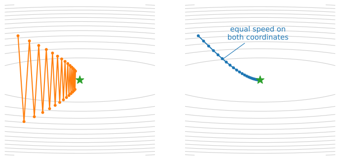
In Section 26.1, stability chained the single step size to the stiffest mode (\(\eta < 2/\lambda_{\max}\)), so the flattest mode advances by only \(\eta\lambda_{\min} \approx 2/\kappa\) per step, which gives a cost linear in \(\kappa\). Now suppose the coordinate axes happen to be the eigendirections, as they are for \(f(\mathbf{x}) = \tfrac12 \mathbf{x}^\top \mathrm{diag}(\boldsymbol{\lambda})\, \mathbf{x}\), and we allow a separate step size \(\eta_i\) per coordinate. Then \(\eta_i = 1/\lambda_i\) contracts every mode to zero in one step: a diagonal matrix of step sizes is a diagonal Newton’s method, and the condition-number dependence is eliminated. This observation motivates the coordinatewise scaling shown in Figure 26.2.1.
Two issues remain. The eigenvalues are unknown and, beyond a fixed quadratic, local curvature varies with the iterate. Stochastic gradients also provide only noisy first-order information. Adaptive methods therefore estimate a useful diagonal rescaling from the observed gradients.
26.2.2.2 AdaGrad and Accumulated Squared Gradients
The first such scheme is AdaGrad (Duchi et al. 2011) (shown in action in Section 9.6). It keeps a running sum of squared gradients per coordinate and divides by its square root:
\[ \mathbf{s}_t = \mathbf{s}_{t-1} + \mathbf{g}_t^2, \qquad \mathbf{x}_{t+1} = \mathbf{x}_t - \frac{\eta}{\sqrt{\mathbf{s}_t} + \epsilon}\; \mathbf{g}_t, \tag{26.2.2}\]
with all operations elementwise and \(\epsilon\) a small constant that keeps the division finite. Two independent derivations motivate this rule.
The metric view. Exercise 2 of Section 26.1 showed that steepest descent is relative to a choice of norm: measuring step length by \(\|\mathbf{d}\|_A = \sqrt{\mathbf{d}^\top A\, \mathbf{d}}\) makes the steepest direction \(-A^{-1}\nabla f\), a preconditioned gradient. AdaGrad is steepest descent in the metric \(A_t = \mathrm{diag}(\sqrt{\mathbf{s}_t})\): it weights each coordinate in proportion to the accumulated evidence \(\sqrt{\sum_{s \le t} g_{s,i}^2}\) that its gradient has been large. Newton would use the true curvature \(\mathrm{diag}(\lambda_i)\); AdaGrad substitutes a first-order proxy based on gradient history (Exercise 1 derives the update from this view).
The regret view, and why the square root. AdaGrad was invented for online convex optimization: convex losses \(f_1, f_2, \ldots\) arrive one at a time, the algorithm must choose \(\mathbf{x}_t\) before observing \(f_t\), and performance is measured by regret, the gap \(\sum_{t=1}^{T} f_t(\mathbf{x}_t) - \min_{\mathbf{x}} \sum_{t=1}^{T} f_t(\mathbf{x})\) between the accumulated loss and that of the best fixed point chosen in hindsight; an algorithm learns, in this sense, when its average regret (regret divided by \(T\)) vanishes as \(T \to \infty\). The problems AdaGrad was built for have sparse features: for example, a bag-of-words model where the coordinate for a rare word receives a nonzero gradient once in ten thousand steps. A global \(\eta_t \propto 1/\sqrt{t}\) decays that rare coordinate’s step size along with everyone else’s, so by the time the rare evidence arrives the step is too small to use it. Per-coordinate accumulation fixes this: coordinate \(i\)’s effective step \(\eta/\sqrt{s_{t,i}}\) decays with its own activity, not with wall-clock time, so rare-but-informative coordinates keep large steps. The square root is what the regret analysis selects: with the per-coordinate rates chosen this way, the accumulated-gradient terms in the regret bound sum to exactly \(\sum_i \sqrt{\sum_t g_{t,i}^2}\), a quantity that can beat the dimension-free \(G\sqrt{T}\) regret of plain SGD by a factor up to \(\sqrt{d}\) when gradients are sparse (Duchi et al. 2011).
The same accumulation is AdaGrad’s defect outside the convex setting. Since \(\mathbf{s}_t\) is cumulative, so the effective step decays like \(\eta/(\sigma\sqrt{t})\) under persistent gradient noise: a Robbins–Monro-style schedule determined by the update definition. On a convex problem this can meet a standard convergence requirement; on a nonconvex objective the iterates may encounter a plateau or saddle region after \(\mathbf{s}_t\) has grown large, when effective steps are close to zero. The cumulative denominator can therefore make later progress impractically slow.
26.2.2.3 RMSProp and Exponential Averaging
RMSProp replaces the all-time sum with an exponential moving average, allowing the scale estimate to respond to recent gradients. RMSProp (Tieleman and Hinton 2012) (shown in action in Section 9.6) keeps
\[ \mathbf{v}_t = \beta_2\, \mathbf{v}_{t-1} + (1 - \beta_2)\, \mathbf{g}_t^2, \qquad \mathbf{x}_{t+1} = \mathbf{x}_t - \frac{\eta}{\sqrt{\mathbf{v}_t} + \epsilon}\; \mathbf{g}_t, \tag{26.2.3}\]
so \(\mathbf{v}_t\) is a weighted average of recent squared gradients with an effective memory of about \(1/(1 - \beta_2)\) steps (\(10\) at RMSProp’s standard decay \(\beta_2 = 0.9\)). The preconditioner now estimates the current gradient scale per coordinate rather than the lifetime total: steps no longer decay to zero by construction, and the method can keep moving when gradient scales change. The corresponding limitation is that exponential decay reduces the influence of rare past gradients, as the counterexample below demonstrates.
26.2.2.4 Adam: Momentum, Second Moments, and Bias Correction
Adam (Kingma and Ba 2015) (shown in action in Section 9.6) combines these components by applying the same exponential averaging to the gradient itself and correcting both averages for their startup bias. The gradient average \(\mathbf{m}_t\) is momentum (Section 26.1.4) in averaged form: where the heavy-ball buffer of that section accumulates gradients, the \((1 - \beta_1)\) factor here makes \(\mathbf{m}_t\) a weighted average of them, the same method up to a rescaling of the step size:
\[ \begin{aligned} \mathbf{m}_t &= \beta_1\, \mathbf{m}_{t-1} + (1 - \beta_1)\, \mathbf{g}_t, \qquad & \hat{\mathbf{m}}_t &= \mathbf{m}_t / (1 - \beta_1^t), \\ \mathbf{v}_t &= \beta_2\, \mathbf{v}_{t-1} + (1 - \beta_2)\, \mathbf{g}_t^2, \qquad & \hat{\mathbf{v}}_t &= \mathbf{v}_t / (1 - \beta_2^t), \\ \mathbf{x}_{t+1} &= \mathbf{x}_t - \eta\; \frac{\hat{\mathbf{m}}_t}{\sqrt{\hat{\mathbf{v}}_t} + \epsilon}, \end{aligned} \tag{26.2.4}\]
with defaults \(\beta_1 = 0.9\), \(\beta_2 = 0.999\), \(\epsilon = 10^{-8}\), and \(\mathbf{m}_0 = \mathbf{v}_0 = \mathbf{0}\). The default \(\beta_2 = 0.999\) gives the second-moment estimate an effective memory of about \(1/(1-\beta_2) = 1000\) steps, a hundred times longer than RMSProp’s customary ten. The bias correction follows by unrolling the recursion. Unroll the recursion:
\[ \mathbf{v}_t = (1 - \beta_2) \sum_{s=1}^{t} \beta_2^{\,t-s}\, \mathbf{g}_s^2 . \]
If the squared-gradient scale is (locally) stationary, \(\mathbb{E}[\mathbf{g}_s^2] = \bar{\mathbf{g}^2}\) for all \(s\), then by the geometric series \(\sum_{s=1}^{t} \beta_2^{\,t-s} = (1 - \beta_2^t)/(1 - \beta_2)\),
\[ \mathbb{E}[\mathbf{v}_t] = (1 - \beta_2)\, \bar{\mathbf{g}^2} \sum_{s=1}^{t} \beta_2^{\,t-s} = \left(1 - \beta_2^t\right) \bar{\mathbf{g}^2}, \tag{26.2.5}\]
so dividing by \(1 - \beta_2^t\) makes \(\hat{\mathbf{v}}_t\) an exactly unbiased estimate of \(\bar{\mathbf{g}^2}\) at every \(t\): the correction factors remove the zero-initialization bias identically at every step. The same computation with \(\beta_1\) handles \(\hat{\mathbf{m}}_t\) (Exercise 2). The transient being corrected is large: at the defaults, \(\mathbf{v}_{10}\) has only about \(1\%\) of its stationary expectation, and the raw ratio \(\mathbf{m}_t/(\sqrt{\mathbf{v}_t} + \epsilon)\) mis-scales early steps by the factor \((1-\beta_1^t)/\sqrt{1-\beta_2^t}\): already \(3.16\) at \(t = 1\), peaking above \(6\times\) near \(t = 12\), because the momentum average saturates in about ten steps while the second-moment average needs about a thousand. Figure 26.2.2 plots the transient and its cancellation.
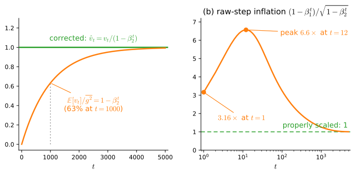
Adam combines three components: RMSProp’s per-coordinate scale estimate, momentum’s variance-averaged direction, and an exact startup correction for both. Near a minimum of a quadratic with diagonal Hessian, the scale estimate obeys \(\sqrt{\hat{v}_i} \approx |g_i| = \lambda_i |x_i|\), so the update on coordinate \(i\) is \(\eta\, g_i / \sqrt{\hat{v}_i} \approx \eta\,\mathrm{sign}(x_i)\): approximately constant-magnitude sign descent, where a diagonal Newton step would move by \(x_i\) itself. The relevant part of the opening argument is the ratio between coordinates: the effective step \(\eta/(\lambda_i |x_i|)\) scales like \(1/\lambda_i\) wherever the \(|x_i|\) are comparable (as at the equal-coordinate start of the comparison below), so stiff coordinates take small steps and flat ones take large steps, estimated from first-order information alone.
26.2.2.5 When Adam Fails to Converge
Adam’s exponentially weighted second moment does not provide a general convergence guarantee, even for convex online problems. Reddi et al. (2018) give the following one-dimensional construction.
Proposition (Adam need not converge). Consider online optimization over the interval \(x \in [-1, 1]\) with the periodic sequence of convex losses
\[ f_t(x) = \begin{cases} C\,x, & t \bmod 3 = 1, \\ -x, & \textrm{otherwise}, \end{cases} \qquad C > 2, \tag{26.2.6}\]
whose gradients over one period sum to \(C - 2 > 0\), so the best fixed point is \(x^\star = -1\). Adam with \(\beta_1 = 0\), \(\beta_2 = 1/(1 + C^2)\), and any step sequence \(\eta_t = \eta/\sqrt{t}\) makes positive net progress each period: its iterates converge to \(x = +1\), where every third loss is maximal, and its average regret does not vanish. (Reddi et al. 2018) extend the construction to \(\beta_1 < \sqrt{\beta_2}\): within that parameter range, a suitable \(C\) defeats any fixed exponential decay.
This proposition is an existence result for a periodic online sequence. It does not say that Adam diverges on every finite dataset or for every practical hyperparameter choice. It identifies a specific obstruction: the exponential second-moment estimate can decrease, causing a coordinate’s effective learning rate to increase. AMSGrad replaces that estimate by a running maximum; its convergence results still require the assumptions stated in the corresponding theorem.
The failure occurs because the effective step on the informative gradient shrinks faster than its information accrues. When the rare large gradient \(C\) occurs, its squared value enters \(\mathbf{v}\): \(v_t\) jumps to nearly \(C^2\), so the corresponding update is normalized by nearly \(C\) and moves the iterate by only \(O(\eta_t)\). Then \(\beta_2\)’s exponential decay reduces its contribution: over the next two steps \(v_t\) collapses back toward \(1\), and the two small \(-1\) gradients each receive much larger effective steps toward the suboptimal boundary. The resulting signed drift repeats every period. This is a different failure from the noise ball of Section 26.1 (which shrinks with the step size): the drift is directed, and the iterate converges to the suboptimal boundary. The AMSGrad modification (Reddi et al. 2018), replaces \(\hat{\mathbf{v}}_t\) by the running maximum \(\tilde{\mathbf{v}}_t = \max(\tilde{\mathbf{v}}_{t-1}, \mathbf{v}_t)\), which makes the per-coordinate step nonincreasing (the large gradient is never forgotten) and restores a convergence guarantee under the assumptions analyzed by Reddi et al. (2018) . The cell runs the construction with \(C = 4\) against AMSGrad and plain projected SGD with the same \(1/\sqrt{t}\) decay:
def online(method, C=4.0, T=15000, alpha=0.5):
    beta2 = 1 / (1 + C * C)                    # the proposition's beta_2
    x, v, vmax, xs = 0.0, 0.0, 0.0, []
    for t in range(1, T + 1):
        g = C if t % 3 == 1 else -1.0          # rare +C, frequent -1
        v = beta2 * v + (1 - beta2) * g * g
        vmax = max(vmax, v)
        if method == 'sgd':
            step = alpha / np.sqrt(t) * g / C
        else:                                  # adam (beta_1 = 0) or amsgrad
            vv = vmax if method == 'amsgrad' else v
            step = alpha / np.sqrt(t) * g / (np.sqrt(vv) + 1e-8)
        x = min(1.0, max(-1.0, x - step))      # project back onto [-1, 1]
        xs.append(x)
    return xs

print('        x_t at t =    30      300     3000    15000     (x* = -1)')
for method in ['adam', 'amsgrad', 'sgd']:
    xs = online(method)
    print(f'{method:8s}' + ''.join(f'{xs[t - 1]:9.3f}'
                                   for t in (30, 300, 3000, 15000)))
x_t at t = 30 300 3000 15000 (x* = -1)
adam 0.745 1.000 1.000 1.000
amsgrad -0.953 -0.985 -0.995 -0.998
sgd -0.954 -0.986 -0.995 -0.998Adam moves to \(+1\) in this construction, while AMSGrad and SGD approach \(-1\). The example is convex, one-dimensional, and has bounded gradients, so it isolates the interaction between exponential forgetting and the periodic gradient sequence. Its pattern should not be identified automatically with rare tokens, rare classes, or occasional loss spikes in ordinary training. The theorem supports the narrower conclusion that vanilla Adam lacks a general convergence guarantee without additional assumptions or modification.
26.2.2.6 Coordinate Scaling on a Diagonal Quadratic
A separate experiment measures the benefit of Adam’s coordinate scaling on an ill-conditioned diagonal quadratic. The cell returns to the ill-conditioned quadratic of Section 26.1 at \(\kappa = 10^3\) and compares tuned gradient descent (the optimal single step \(\eta^\star = 2/(\lambda_{\min} + \lambda_{\max})\)) against hand-rolled Adam, printing Adam’s effective per-coordinate steps \(\eta/(\sqrt{\hat{\mathbf{v}}_t} + \epsilon)\) as it runs:
lam = np.array([1.0, 1000.0])                  # kappa = 1000
f = lambda x: 0.5 * (lam * x * x).sum()

def race(optimizer, eta, K=20000, tol=1e-8):
    x, m, v, hit = np.array([1.0, 1.0]), np.zeros(2), np.zeros(2), None
    for k in range(1, K + 1):
        g = lam * x
        if optimizer == 'gd':
            x = x - eta * g
        else:                                  # adam, the update of the text
            m = 0.9 * m + 0.1 * g
            v = 0.999 * v + 0.001 * g * g
            step = eta / (np.sqrt(v / (1 - 0.999**k)) + 1e-8)
            if k in (1, 100, 1000):
                print(f'   k = {k:4d}: effective steps {step.round(6)}')
            x = x - step * (m / (1 - 0.9**k))
        if hit is None and f(x) < tol:
            hit = k
    return hit

hit = race('gd', 2 / lam.sum())
print(f'GD, optimal single eta = {2 / lam.sum():.1e}: f < 1e-8 at k = {hit}')
print('Adam, eta = 0.01:')
print(f'Adam reaches f < 1e-8 at k = {race("adam", 0.01)}')
GD, optimal single eta = 2.0e-03: f < 1e-8 at k = 6160
Adam, eta = 0.01:
k = 1: effective steps [1.e-02 1.e-05]
k = 100: effective steps [1.6534e-02 1.7000e-05]
k = 1000: effective steps [6.5755e-02 6.6000e-05]
Adam reaches f < 1e-8 at k = 344Gradient descent with the optimal single step needs \(6160\) iterations, and the \((\kappa-1)/(\kappa+1)\) contraction law of Section 26.1 predicts that count exactly: with \(\eta^\star\) both coordinates contract by \(\rho = 999/1001\) per step, so \(f_k = 500.5\,\rho^{2k}\) crosses \(10^{-8}\) at \(k = 6159.07\), making \(6160\) the first iterate under tolerance. Adam gets there in \(344\). The printed effective steps say why: from the first iteration Adam’s step on the stiff coordinate is \(10^{-5}\) and on the flat coordinate \(10^{-2}\), the \(1000\times\) ratio of the eigenvalues, reconstructed from gradient magnitudes alone, with no eigendecomposition and no Hessian. Both coordinates then approach zero at comparable rates, as shown in the right panel of Figure 26.2.1. The diagonal scaling reduces the coordinatewise imbalance.
This comparison has important limitations. On this problem, exact preconditioning is available: Newton’s method solves it in one step, and even a fixed diagonal \(\eta_i = 1/\lambda_i\) needs no adaptivity at all. Adam estimates coordinate scales continuously from noisy first-order data at \(O(d)\) cost. And the approximation is crude: \(\sqrt{\hat{\mathbf{v}}}\) conflates curvature with gradient noise (both inflate squared gradients), the diagonal ignores every off-axis correlation (rotate this quadratic by \(45°\) and per-coordinate rescaling loses most of its effect), and the Reddi construction gives an adversarial sequence for which the estimate fails. Adaptive methods trade curvature fidelity for per-step cost. The final section compares diagonal scaling with more structured preconditioners.
26.2.3 Decoupled Weight Decay
26.2.3.1 The Penalty Gradient Goes Through the Preconditioner
Under SGD, adding \(\tfrac{\lambda}{2}\|\mathbf{w}\|^2\) to the loss, get \(\lambda \mathbf{w}\) added to the gradient. produces the same update whether implemented as an objective penalty or as direct parameter shrinkage:
\[ \mathbf{w}_{t+1} = \mathbf{w}_t - \eta\,(\mathbf{g}_t + \lambda \mathbf{w}_t) = (1 - \eta\lambda)\, \mathbf{w}_t - \eta\, \mathbf{g}_t . \]
Under Adam they are not, as the following derivation shows. Feed the penalized gradient through Equation 26.2.4 and look at the decay term alone (take \(\beta_1 = 0\) for clarity, so the update is \(-\eta\,(\mathbf{g}_t + \lambda\mathbf{w}_t)/(\sqrt{\hat{\mathbf{v}}_t} + \epsilon)\)): the shrinkage applied to coordinate \(i\) is
\[ \textrm{$\ell_2$ through Adam:}\quad \frac{\eta\,\lambda}{\sqrt{\hat{v}_{t,i}} + \epsilon}\; w_{t,i} \qquad \textrm{versus} \qquad \textrm{decoupled:}\quad \eta\,\lambda\, w_{t,i} . \tag{26.2.7}\]
The preconditioner divides the penalty gradient as well as the loss gradient, so the regularization strength is no longer a constant of the problem: it varies per coordinate and over time, inversely with the gradient scale. A weight whose loss gradients are large or noisy (large \(\hat{v}_i\)) receives weaker shrinkage; a weight with small gradients receives stronger shrinkage. The Gaussian-prior MAP interpretation in Section 27.3 and the norm-constraint interpretation in Section 26.4.4.5 both assume one \(\lambda\) for all coordinates. Coupling the penalty to Adam’s preconditioner produces a coordinate- and time-dependent coefficient, so those interpretations no longer apply directly.
AdamW (Loshchilov and Hutter 2019) restores the intended semantics by decoupling: the loss gradient goes through the preconditioner, the decay does not,
\[ \mathbf{w}_{t+1} = (1 - \eta\lambda)\, \mathbf{w}_t - \eta\; \frac{\hat{\mathbf{m}}_t}{\sqrt{\hat{\mathbf{v}}_t} + \epsilon}, \]
which is verbatim the SGD shrinkage \((1 - \eta\lambda)\), applied uniformly. An empirical finding motivated the fix: \(\ell_2\)-regularized Adam generalized worse than SGD with weight decay, and decoupling closed the gap. That finding is downstream of exactly the per-coordinate distortion in Equation 26.2.7. The cell isolates that distortion: two weights whose loss gradients are pure noise (so decay is the only systematic force) at very different noise scales, \(\sigma = (10, 0.1)\).
sig, alpha, lam_wd, T = np.array([10.0, 0.1]), 1e-3, 0.1, 4000

def decay_race(decoupled, seed=0):
    rg = np.random.default_rng(seed)
    w, m, v = np.array([1.0, 1.0]), np.zeros(2), np.zeros(2)
    for t in range(1, T + 1):
        g = sig * rg.standard_normal(2)        # loss gradient: pure noise
        if not decoupled:
            g = g + lam_wd * w                 # l2 penalty inside the gradient
        m, v = 0.9 * m + 0.1 * g, 0.999 * v + 0.001 * g * g
        w = w - alpha * (m / (1 - 0.9**t)) / (np.sqrt(v / (1 - 0.999**t)) + 1e-8)
        if decoupled:
            w = w - alpha * lam_wd * w         # decay outside the preconditioner
    return w

print('per-step decay rate, l2 through Adam (alpha*lam/sigma_i):',
      (alpha * lam_wd / sig).round(6))
print('per-step decay rate, AdamW (uniform):                    ',
      alpha * lam_wd)
print(f'|w| after {T} steps,  Adam + l2: {np.abs(decay_race(False)).round(4)}')
print(f'|w| after {T} steps,  AdamW    : {np.abs(decay_race(True)).round(4)}')
print(f'AdamW prediction (1 - alpha*lam)^T = {(1 - alpha * lam_wd)**T:.4f}')
per-step decay rate, l2 through Adam (alpha*lam/sigma_i): [1.e-05 1.e-03]
per-step decay rate, AdamW (uniform): 0.0001
|w| after 4000 steps, Adam + l2: [0.9677 0.0235]
|w| after 4000 steps, AdamW : [0.6681 0.6598]
AdamW prediction (1 - alpha*lam)^T = 0.6703Under \(\ell_2\)-through-Adam the noisy coordinate has decayed from \(1\) to only \(0.968\) after \(4000\) steps while the quiet coordinate has collapsed to \(0.024\): effective decay rates of \(10^{-5}\) versus \(10^{-3}\), the predicted \(\eta\lambda/\sigma_i\), an induced \(100\times\) disparity. AdamW shrinks both to \(\approx 0.66\), within \(2\%\) of the pure-decay prediction \((1 - \eta\lambda)^T = 0.6703\): one \(\lambda\) with one meaning. (A subtlety about fixed points: at a deterministic stationary point, coupled Adam is stationary exactly where SGD with \(\ell_2\) is, at \(\nabla L + \lambda\mathbf{w} = \mathbf{0}\), while AdamW’s stationary points sit elsewhere; Exercise 4 derives both conditions and explains why decoupling matters in the noisy, never-stationary training regime, where the sequence of updates matters in addition to fixed points.) In the major libraries, AdamW and Adam with a weight_decay flag implement two different regularizers: the former is the decoupled update exactly, the latter the coupled Equation 26.2.7.
26.2.4 Schedules and Warmup
26.2.4.1 What Decay Does, and Which Shape
A learning-rate schedule is a sequence \(\eta_t\) (the main book surveys the common ones in Section 9.8), and the relevant mathematical tradeoff was already proved in Section 26.1: on the persistent-noise quadratic analyzed there, a constant step leaves SGD at a noise floor proportional to \(\eta\) Equation 26.1.17. Under the assumptions of the Robbins–Monro theorem, decay satisfying Equation 26.1.18 can converge to the optimum, whereas an undersized constant in \(\eta_k = c/k\) can degrade the rate class.
Add to this the Ghadimi–Lan prescription of this section: for a fixed nonconvex budget \(K\), a constant \(\eta \propto 1/\sqrt{K}\) is already minimax-optimal, meaning no method that sees only the same unbiased, bounded-variance gradient oracle can guarantee a better worst-case rate than the \(K^{-1/2}\) it achieves; the matching lower bound is due to Arjevani et al. (2023) . In this analysis, decay has a specific role: it lowers the noise floor, at a cost in transient progress, and beyond convex problems no theorem ranks one decay shape against another. The following discussion distinguishes proved statements from empirical design choices. Three common schedules, drawn in Figure 26.2.3, are these:
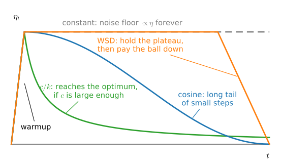
Cosine decay (Loshchilov and Hutter 2016) sets \(\eta_t = \tfrac12 \eta_0 (1 + \cos(\pi t / K))\): a smooth descent from \(\eta_0\) to \(0\) with most of its time spent at moderate steps and a long, gentle tail. It satisfies no optimality theorem; it is popular because it has one parameter (\(\eta_0\)), no kinks to tune, and is widely used across training budgets. Warmup–stable–decay (WSD) (Hu et al. 2024) holds \(\eta_0\) constant for most of the run and decays only in a final fraction (often the last \(10\)–\(20\%\)). Its practical appeal is operational: the long constant plateau means checkpoints from one run can be re-decayed to any budget, rather than committing to \(K\) at launch. On the quadratic model, the constant plateau permits rapid transient progress but retains a noise floor; the final decay reduces that floor. This interpretation does not prove that the plateau is beneficial on a neural-network loss. Its practical advantages and typical final-decay fraction are empirical choices. The cell compares the shapes at equal budget on the noisy quadratic, where the noise floor is exact, printing the loss at \(80\%\) of the budget and at the end:
lam_s, sigma, K, eta0 = 1.0, 1.0, 2000, 0.3

def run_schedule(eta_fn, seeds=200):
    at80, final = [], []
    for s in range(seeds):
        rg, x = np.random.default_rng(s), 3.0
        for k in range(K):
            x = x - eta_fn(k) * (lam_s * x + sigma * rg.standard_normal())
            if k == int(0.8 * K) - 1:
                at80.append(0.5 * lam_s * x * x)
        final.append(0.5 * lam_s * x * x)
    return np.mean(at80), np.mean(final)

schedules = [
    ('constant', lambda k: eta0),
    ('c/k decay', lambda k: eta0 / (1 + k / 50)),
    ('cosine', lambda k: 0.5 * eta0 * (1 + np.cos(np.pi * k / K))),
    ('WSD 80/20', lambda k: eta0 if k < 0.8 * K else eta0 * (K - k) / (0.2 * K)),
]
print(f'         E f at 80% budget   E f at end     (floor ~ '
      f'{eta0 * sigma**2 / (2 * (2 - eta0 * lam_s)):.3f})')
for name, fn in schedules:
    m80, mK = run_schedule(fn)
    print(f'{name:10s}    {m80:9.2e}      {mK:9.2e}')
E f at 80% budget E f at end (floor ~ 0.088)
constant 9.53e-02 9.19e-02
c/k decay 2.82e-03 1.94e-03
cosine 8.71e-03 1.58e-03
WSD 80/20 9.53e-02 5.48e-03The constant run sits on its floor at both checkpoints (\(9.5\) and \(9.2 \times 10^{-2}\), against the printed prediction \(\eta\sigma^2/(2(2 - \eta\lambda)) \approx 0.088\)), while every decaying schedule ends one to two orders lower. The instructive row is WSD: at \(80\%\) of the budget it is still on the constant’s floor (\(9.5 \times 10^{-2}\), equal to the constant row to every printed digit, since the two runs are the same trajectory until the decay begins), then the final \(400\) steps drop it by a factor of \(17\). All of WSD’s visible improvement arrives in the decay phase. On this quadratic, cosine’s longer tail of small steps gives the lower final error (\(1.6 \times 10^{-3}\)); this quadratic does not evaluate WSD’s operational benefits, such as re-decayable checkpoints or allocating more steps to a large-learning-rate phase.
26.2.4.2 Warmup for an Estimated Preconditioner
The plotted schedules begin with warmup: \(\eta_t\) is ramped linearly from approximately zero over an initial interval (Goyal et al. 2017). Warmup is a common empirical device for both SGD and adaptive methods; the arguments below explain why it can help, not why every model requires it or how long it must last.
First, the preconditioner is estimated from very few samples. At \(t = 1\), \(\hat{\mathbf{v}}_1 = \mathbf{g}_1^2\): the per-coordinate rescaling is estimated from a single sample, and bias correction makes it unbiased, not accurate. The step direction \(\hat{\mathbf{m}}_1/(\sqrt{\hat{\mathbf{v}}_1} + \epsilon) = \mathrm{sign}(\mathbf{g}_1)\) produces full-magnitude movement on every coordinate, including ones whose lone observed gradient was dominated by noise. The exponential weights have a characteristic timescale \(1/(1 - \beta_2) = 1000\) steps, although the useful warmup length depends on the gradient distribution and batch size. Ramping \(\eta\) while estimates accumulate can reduce the effect of noisy early rescaling. (This diagnosis can also be read off Figure 26.2.2: the correction fixes the mean of the early estimate; its variance decreases only as observations accumulate.)
Second, local curvature may change rapidly near initialization. A target step that is stable later in training can violate an early local stability bound. Warmup reduces the proposed step during this transient. Edge-of-stability measurements motivate this explanation, but they do not yield a universal warmup theorem, duration, or schedule for deep networks.
A separate, architecture-dependent mechanism is rapid early change in activation and back-propagated gradient scales. Warmup can damp the resulting parameter changes, but this mechanism is not implied by the preconditioner or quadratic-curvature analyses above.
26.2.5 Variance Reduction for Finite Sums
Minibatching reduces variance by averaging more examples, but a fixed-size minibatch still has noise at the optimum. A finite training set offers another possibility: reuse information from earlier gradients as a control variate. Write the empirical objective as
\[ F(\mathbf x)=\frac1n\sum_{i=1}^n f_i(\mathbf x). \]
At a reference point \(\widetilde{\mathbf x}\), compute the full gradient \(\widetilde{\boldsymbol\mu}=\nabla F(\widetilde{\mathbf x})\). The SVRG estimator at the current point is
\[ \mathbf v_i(\mathbf x) =\nabla f_i(\mathbf x)-\nabla f_i(\widetilde{\mathbf x}) +\widetilde{\boldsymbol\mu}. \tag{26.2.8}\]
For a uniformly sampled index,
\[ \mathbb E_i[\mathbf v_i(\mathbf x)] =\nabla F(\mathbf x)-\nabla F(\widetilde{\mathbf x}) +\nabla F(\widetilde{\mathbf x}) =\nabla F(\mathbf x), \]
so the estimator is unbiased. Its advantage is not the mean but the variance: when \(\mathbf x\) is close to the snapshot, the two component gradients are highly correlated and their difference is much less variable than either one. After an inner loop moves too far from the snapshot, refresh the full gradient and repeat. Under smooth strong convexity, this mechanism yields geometric convergence with a fixed step size, rather than SGD’s fixed-step noise floor (Bottou et al. 2018).
The cell compares SVRG with SGD on ridge regression. One SVRG epoch pays \(n\) component-gradient equivalents for the full gradient and two per inner step; SGD receives the same total budget of \(3n\) component gradients per reported epoch. Both use a fixed step size, so the comparison isolates the control variate rather than a schedule.
rng = np.random.default_rng(4)
n_vr, d_vr = 300, 12
X_vr = rng.standard_normal((n_vr, d_vr))
w_true_vr = rng.standard_normal(d_vr)
y_vr = X_vr @ w_true_vr + 0.5 * rng.standard_normal(n_vr)
lam_vr = 0.1
H_vr = X_vr.T @ X_vr / n_vr + lam_vr * np.eye(d_vr)
w_star_vr = np.linalg.solve(H_vr, X_vr.T @ y_vr / n_vr)

def component_grad(w, i):
    return X_vr[i] * (X_vr[i] @ w - y_vr[i]) + lam_vr * w

def full_grad(w):
    return X_vr.T @ (X_vr @ w - y_vr) / n_vr + lam_vr * w

def objective_vr(w):
    return (0.5 * np.mean((X_vr @ w - y_vr)**2)
            + 0.5 * lam_vr * (w @ w))

eta_vr, epochs_vr = 0.05, 20
snapshot, gaps_svrg = np.zeros(d_vr), []
for _ in range(epochs_vr):
    mean_grad = full_grad(snapshot)
    w = snapshot.copy()
    for _ in range(n_vr):
        i = rng.integers(n_vr)
        v = component_grad(w, i) - component_grad(snapshot, i) + mean_grad
        w -= eta_vr * v
    snapshot = w
    gaps_svrg.append(objective_vr(snapshot) - objective_vr(w_star_vr))

rng_sgd = np.random.default_rng(5)
w_sgd, gaps_sgd = np.zeros(d_vr), []
for _ in range(epochs_vr):
    for _ in range(3 * n_vr):               # same component-gradient budget
        i = rng_sgd.integers(n_vr)
        w_sgd -= eta_vr * component_grad(w_sgd, i)
    gaps_sgd.append(objective_vr(w_sgd) - objective_vr(w_star_vr))

d2l.plot(np.arange(1, epochs_vr + 1), [gaps_sgd, gaps_svrg],
         'equal-budget epoch', 'optimality gap',
         legend=['SGD, fixed step', 'SVRG, fixed step'], yscale='log')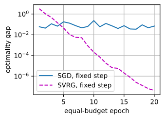
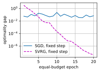
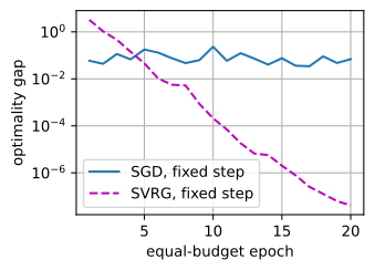
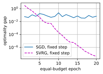
SGD reduces the objective quickly at first, but its constant-step iterates continue to fluctuate around the optimum. SVRG incurs the cost of its snapshots and then drives the gap down geometrically on this finite, strongly convex problem. The result does not establish that SVRG universally outperforms SGD: full passes are expensive on enormous or streaming datasets, the linear-rate theorem uses finite-sum smoothness and convexity, and stale control variates are less effective when the objective changes during training.
SAGA removes the periodic full-gradient pass by storing the most recently seen gradient for every example and using their table average as the control variate. It spends one new component gradient per step but stores \(O(nd)\) numbers in the literal form (structure can reduce this for generalized linear models). SARAH-style estimators update the control variate recursively. The methods share one control-variate principle: correlate a noisy new estimate with a stored estimate whose mean is known, subtract the shared noise, and add the known mean back.
Variance reduction is distinct from momentum. Momentum averages gradients across recent iterates and can reduce high-frequency noise, but its moving average is generally biased for the gradient at the current point. SVRG and SAGA engineer an estimator that is unbiased at the current point and whose variance shrinks as the optimization converges.
26.2.6 Preconditioners Beyond Diagonal Scaling
Each method in this section chooses a matrix \(B_t\) to multiply the gradient, \(\mathbf{x}_{t+1} = \mathbf{x}_t - \eta\, B_t\, \mathbf{g}_t\). Gradient descent answers \(B = I\); Newton answers \(B = (\nabla^2 f)^{-1}\) at \(O(d^3)\); Adam answers with a diagonal estimated from gradient history at \(O(d)\). Between the diagonal and the full inverse Hessian are structured approximations. Matrix-valued layer structure makes some of them affordable: a network’s parameters occur in layers of matrices, so an approximation can discard curvature between layers while retaining structured curvature within each layer.
Kronecker-factored curvature (K-FAC) (Martens and Grosse 2015) treats each layer’s weight matrix \(W \in \mathbb{R}^{m \times n}\) separately and approximates its block of the Fisher information matrix, the outer-product curvature \(\mathbb{E}[\nabla \log p\, \nabla \log p^\top]\) that Section 27.3 introduced. The word curvature is precise here: for log-likelihood losses the Fisher equals the Gauss–Newton matrix, the PSD part of the Hessian obtained by dropping the second-derivative terms of the network (Martens and Grosse 2015). K-FAC’s approximation is a Kronecker product \(A \otimes G\) (the block matrix whose \((i,j)\) block is \(a_{ij}\, G\)), where \(A = \mathbb{E}[\mathbf{a}\mathbf{a}^\top]\) is the second moment of the layer’s inputs and \(G = \mathbb{E}[\boldsymbol{\delta}\boldsymbol{\delta}^\top]\) that of the gradients at its outputs. The factorization is exact if the layer’s inputs and output-gradients are statistically independent under the model’s distribution; that independence is the approximation, and in trained networks it holds only approximately. The Kronecker inverse identity reduces the cost. Writing \(\mathrm{vec}(V)\) for the vector obtained by stacking the columns of the layer’s gradient matrix \(V\),
\[ (A \otimes G)^{-1}\, \mathrm{vec}(V) \;=\; \mathrm{vec}\left(G^{-1}\, V\, A^{-1}\right), \tag{26.2.9}\]
Thus, preconditioning by a curvature matrix with \((mn)^2\) entries requires two smaller inverses, of sizes \(n \times n\) and \(m \times m\). Preconditioning by the Fisher gives the natural gradient (Amari 1998), steepest descent when distance is measured between the distributions the parameters define rather than between parameter vectors, the metric view of AdaGrad again, with the Fisher as the metric. Shampoo (Gupta et al. 2018) keeps the same two-sided structure but builds the factors AdaGrad-style from accumulated gradient statistics, preconditioning \(V \mapsto L^{-1/4} V R^{-1/4}\) with \(L = \sum_t V_t V_t^\top\) and \(R = \sum_t V_t^\top V_t\), a two-sided matrix cousin of 1. It is a cousin rather than a strict generalization: restricting \(L, R\) to their diagonals normalizes entry \((i,j)\) by the factored \((l_i r_j)^{1/4}\) of its row and column statistics, not by AdaGrad’s per-entry root, and the precise relation is an inequality (the Kronecker root \(L^{1/4} \otimes R^{1/4}\) upper-bounds the full-matrix AdaGrad preconditioner (Gupta et al. 2018)). Muon (Jordan et al. 2024) takes the limiting view: rather than estimate second moments at all, it replaces each layer’s momentum matrix by its nearest orthogonal matrix, the polar factor \(UV^\top\) of the SVD, computed by the Newton–Schulz iteration demonstrated in Section 24.3. This whitens the update’s spectrum directly: every singular direction of the update moves at the same rate, per-direction step equalization where Adam manages only per-coordinate.
The resulting hierarchy is: diagonal (Adam, \(O(d)\)) \(\to\) per-layer Kronecker factors (K-FAC) \(\to\) per-layer full-matrix roots (Shampoo) \(\to\) per-layer spectral normalization (Muon) \(\to\) full second order (Newton, unreachable). Each level represents more structure and requires more per-step arithmetic. The practical choice depends on hardware cost as well as approximation quality. The same matching of step size to geometry also extends across model sizes: the maximal-update parametrization (muP) (Yang and Hu 2021) derives how per-layer learning rates must scale with width so that one tuned \(\eta\) transfers from a small model to a large one.
26.2.7 Summary
- The Ghadimi–Lan theorem extends the no-convexity guarantee to SGD: with \(\eta \le 1/L\) the descent lemma survives in expectation with a variance term \(\tfrac{L}{2}\eta^2\sigma^2\) per step, and at the balanced \(\eta \propto 1/\sqrt{K}\) a random iterate satisfies \(\mathbb{E}\|\nabla f\|^2 = O(\sigma\sqrt{L\Delta/K})\). Noise turns the deterministic \(1/K\) rate into \(K^{-1/2}\), and the guarantee is for a random iterate (the best one cannot be identified from noisy evaluations).
- Per-coordinate step sizes address \(\kappa\) directly: on a diagonal quadratic, \(\eta_i = 1/\lambda_i\) removes the condition number entirely. AdaGrad is steepest descent in the metric \(\mathrm{diag}(\sqrt{\sum_t \mathbf{g}_t^2})\), built for sparse gradients, but its cumulative denominator can drive steps toward zero and make progress impractically slow on persistent noisy or nonconvex problems; RMSProp substitutes an EMA; Adam adds momentum and exact bias correction: \(\mathbb{E}[\mathbf{v}_t] = (1 - \beta_2^t)\,\bar{\mathbf{g}^2}\) under stationarity, so dividing by \(1 - \beta_2^t\) cancels the zero-initialization deficit identically.
- Vanilla Adam is not guaranteed to converge in general, even on convex problems. In the periodic Reddi–Kale–Kumar online construction, Adam converges to the wrong boundary because the effective step on a large gradient shrinks too rapidly. AMSGrad’s running maximum addresses that mechanism under its theorem assumptions. This existence result does not predict failure on every finite-data problem. On the \(\kappa = 10^3\) quadratic used here, Adam reconstructs the \(1000\times\) eigenvalue ratio from gradient magnitudes alone and requires \(18\times\) fewer iterations than optimally tuned GD in this experiment.
- Coupling an \(\ell_2\) penalty to Adam produces coordinate-dependent shrinkage: its coefficient is \(\eta\lambda/(\sqrt{\hat{v}_i} + \epsilon)\) per coordinate. AdamW decouples the decay from the preconditioner, restoring the uniform \((1 - \eta\lambda)\) that the MAP-prior and norm-constraint readings of \(\lambda\) presuppose.
- Schedules balance the noise floor (\(\propto \eta\)) against transient progress; beyond convexity no theorem ranks decay shapes. Cosine spends a long small-step tail; WSD stays on the constant-step floor until a final decay phase reduces it sharply, as illustrated on a noisy quadratic. Warmup is an empirical response to early transients: at small \(t\) the preconditioner is estimated from few gradients (unbiased \(\ne\) accurate), while activation scales and local curvature may change rapidly. Its useful duration is model-dependent.
- On finite-sum objectives, SVRG subtracts a component gradient at a snapshot and adds the snapshot’s full gradient, producing an unbiased control-variate estimator whose variance shrinks near the snapshot. SAGA replaces full-gradient refreshes by a table of stored component gradients. These methods can reach linear fixed-step convergence under smooth strong convexity, but require repeated access to a finite dataset.
- Between Adam’s diagonal approximation and Newton’s full inverse lies a preconditioning ladder: K-FAC’s Kronecker-factored Fisher (natural gradient at two small inverses via \((A \otimes G)^{-1}\mathrm{vec}(V) = \mathrm{vec}(G^{-1}VA^{-1})\)), Shampoo’s two-sided full-matrix roots, Muon’s Newton–Schulz orthogonalization of momentum, each rung exploiting the fact that parameters come in matrices.
26.2.8 Exercises
- AdaGrad from the metric view. Exercise 2 of Section 26.1 showed that the steepest descent direction under the norm \(\|\mathbf{d}\|_A = \sqrt{\mathbf{d}^\top A \mathbf{d}}\) is proportional to \(-A^{-1}\nabla f\). Set \(A_t = \mathrm{diag}\bigl(\sqrt{\mathbf{s}_t}\bigr) + \epsilon I\) with \(\mathbf{s}_t = \sum_{s \le t} \mathbf{g}_s^2\) and recover
- Why is \(A_t\) built from \(\sqrt{\mathbf{s}_t}\) rather than \(\mathbf{s}_t\)? (Two answers: match the units of a curvature, since squared gradients have the wrong dimensions, and check which choice makes the effective step on a coordinate with i.i.d. noise decay like the Robbins–Monro-compatible \(1/\sqrt{t}\) rather than the too-fast \(1/t\).)
- Bias correction for the first moment. Repeat the computation of Equation 26.2.5 for \(\mathbf{m}_t = \beta_1 \mathbf{m}_{t-1} + (1-\beta_1)\mathbf{g}_t\) under \(\mathbb{E}[\mathbf{g}_s] = \bar{\mathbf{g}}\), obtaining \(\mathbb{E}[\mathbf{m}_t] = (1 - \beta_1^t)\,\bar{\mathbf{g}}\). Then compute the scale of uncorrected Adam’s first step: with \(\mathbf{m}_1 = (1-\beta_1)\mathbf{g}_1\) and \(\mathbf{v}_1 = (1-\beta_2)\mathbf{g}_1^2\), show the raw ratio \(\mathbf{m}_1/\sqrt{\mathbf{v}_1}\) has magnitude \((1-\beta_1)/\sqrt{1-\beta_2} \approx 3.16\) at the defaults. Finally, find (numerically or by calculus) where the inflation factor \((1-\beta_1^t)/\sqrt{1-\beta_2^t}\) peaks and how large it gets, and explain, from the two averaging timescales \(1/(1-\beta_1)\) and \(1/(1-\beta_2)\), why the peak sits where it does.
- The Reddi example by hand. Take \(C = 4\), \(\beta_1 = 0\), \(\beta_2 = 1/17\), a fixed step \(\eta_t = \eta\), and an iterate \(x\) in the interior of \([-1, 1]\) with \(v\) at its period-limit value. Compute the three Adam updates of one period of 2 and show the net displacement over the period is positive (toward the wrong endpoint) for small \(\eta\). Where exactly does the factor \(\sqrt{v} \approx C\) reduce the informative step?
- Coupled versus decoupled fixed points. For \(L(\mathbf{w}) = \tfrac12 (\mathbf{w} - \mathbf{w}_0)^\top
\mathrm{diag}(h_1, h_2) (\mathbf{w} - \mathbf{w}_0)\) with \(h = (100, 1)\) and deterministic gradients, write the stationarity conditions of (a) Adam on \(L + \tfrac{\lambda}{2}\|\mathbf{w}\|^2\) and
- AdamW on \(L\). Show that (a) demands \(\nabla L + \lambda\mathbf{w} = \mathbf{0}\) (the same point as SGD with \(\ell_2\)), while (b) demands \(\nabla L_i = -\lambda w_i (\sqrt{\hat{v}_i} + \epsilon)\), a different point. Reconcile this with the section’s cell: in the noisy, never-stationary regime, which of the two updates applies the uniform per-step shrinkage, and why is that the property that matters during training?
- Where \(\epsilon\) matters. On the \(\kappa = 10^3\) quadratic of the
#adaptive-stochastic-methods-adam-vs-gdcell, sweep \(\epsilon \in \{10^{-12}, 10^{-8}, 10^{-4}, 10^{-2}, 10^{-1}\}\) and record iterations to \(f < 10^{-8}\). Explain the two regimes you find: \(\epsilon\) is invisible while \(\sqrt{\hat{v}_i} \gg \epsilon\), and it converts Adam into plain (momentum) SGD with step \(\eta/\epsilon\) once gradients shrink below it. Which coordinate’s gradients cross that threshold first, and what does \(\epsilon\) therefore control near convergence? - The optimal constant step, exactly. For the noisy scalar quadratic of the
#adaptive-stochastic-methods-schedulescell, iterate the noise-ball recursion of Section 26.1 to get the exact finite-horizon loss \(\mathbb{E}[x_K^2] = (1-\eta\lambda)^{2K} x_0^2 + \bigl(1 - (1-\eta\lambda)^{2K}\bigr)\, \eta\sigma^2/(\lambda(2-\eta\lambda))\). For a fixed budget \(K\), show the minimizing constant step scales like \(\eta^\star = \Theta(\log K / K)\) (balance the exponential transient against the linear-in-\(\eta\) floor), not like the \(1/\sqrt{K}\) of the Ghadimi–Lan prescription, and explain why there is no contradiction (strong convexity versus the nonconvex worst case). Verify your \(\eta^\star\) numerically against a grid search at \(K = 2000\). - AMSGrad’s monotone steps. Show that with the running maximum \(\tilde{\mathbf{v}}_t = \max(\tilde{\mathbf{v}}_{t-1}, \mathbf{v}_t)\) the effective per-coordinate step \(\eta_t/\sqrt{\tilde{v}_{t,i}}\) is nonincreasing in \(t\) whenever \(\eta_t\) is, and explain in one sentence why this property blocks the drift mechanism of
- Then modify the
#adaptive-stochastic-methods-reddicell to interpolate: replace the hard max by \(\tilde{v}_t = \max(\gamma\tilde{v}_{t-1}, v_t)\) and find the largest forgetting factor \(\gamma < 1\) at which the drift to \(+1\) reappears.
- Then modify the
- SVRG unbiasedness and cost. Prove the conditional unbiasedness of
- Count component-gradient evaluations in one epoch of the cell, then vary the inner-loop length from \(n/2\) to \(4n\). Explain the tradeoff between amortizing the snapshot gradient and letting the control variate become stale.
26.2.9 Discussions
This section connects the chapter’s analysis with commonly used training optimizers. The main book shows the methods in action (Section 9.3 and Section 9.4 for stochastic descent, Section 9.5 for velocity, Section 9.6 for the adaptive family, Section 9.8 for schedules), while the Ghadimi–Lan rate, the diagonal-metric derivation, the bias-correction identity, the Reddi counterexample, and the decoupling algebra proved here provide the mathematical basis for those algorithms. Within this part, Section 26.1 supplied the required results (descent lemma, \(\kappa\), minibatch variance, noise ball); Section 26.3 explains which guarantees return when convexity does; and the stationary-distribution view of constant-step SGD, the noise ball as an invariant measure, is developed further with the SDE analysis of Chapter 29.
Further connections are useful after the main derivations: the MAP interpretation of weight decay appears in Section 27.3, its norm-constraint interpretation in Section 26.4.4.5, and structured preconditioners use the matrix factorizations of Section 24.3.