%matplotlib inline
from d2l import torch as d2l
import gymnasium as gym
import numpy as np
import torch
from torch import nn
torch.set_num_threads(1)15.4 Deep Q-Networks
A Deep Q-Network (DQN) replaces the tabular action-value function of Q-learning with a neural network (Mnih et al. 2013, 2015). Unlike supervised regression, its bootstrapped targets depend on the function being trained. Consecutive transitions are correlated, and data in a replay buffer may have been collected by older policies. Together, function approximation, bootstrapping, and off-policy data can make value learning unstable.
DQN addresses two of these interactions with an experience-replay buffer and a target network. We introduce both mechanisms on CartPole, ablate the target network, and compare learned values with bounds implied by the task. The final part measures maximization bias and derives Double DQN, which separates action selection from evaluation.
%matplotlib inline
from d2l import jax as d2l
from flax import nnx
import gymnasium as gym
import jax
from jax import numpy as jnp
import numpy as np
import optax
We again use CartPole with discount \(0.99\), but specify the training budget as \(50{,}000\) environment steps because episode length changes as the policy improves. The agent takes one gradient step after every two environment steps. Its Q-network maps a state to one value per action, and the greedy action is the corresponding argmax.
gamma, num_env_steps, num_seeds = 0.99, 50_000, 3
buffer_size, batch_size, lr = 200_000, 128, 1e-3
train_freq, sync_every, warmup, grad_clip = 2, 250, 1_000, 10.0
epsilon = d2l.linear_schedule(1.0, 0.05, 10_000)
if tab.selected('pytorch'):
    def make_qnet():
        return nn.Sequential(nn.Linear(4, 128), nn.ReLU(),
                             nn.Linear(128, 128), nn.ReLU(),
                             nn.Linear(128, 2))
if tab.selected('jax'):
    def make_qnet(rngs):
        return nnx.Sequential(nnx.Linear(4, 128, rngs=rngs), jax.nn.relu,
                              nnx.Linear(128, 128, rngs=rngs), jax.nn.relu,
                              nnx.Linear(128, 2, rngs=rngs))
gamma, num_env_steps, num_seeds = 0.99, 50_000, 3
buffer_size, batch_size, lr = 200_000, 128, 1e-3
train_freq, sync_every, warmup, grad_clip = 2, 250, 1_000, 10.0
epsilon = d2l.linear_schedule(1.0, 0.05, 10_000)
if tab.selected('pytorch'):
def make_qnet():
return nn.Sequential(nn.Linear(4, 128), nn.ReLU(),
nn.Linear(128, 128), nn.ReLU(),
nn.Linear(128, 2))
if tab.selected('jax'):
def make_qnet(rngs):
return nnx.Sequential(nnx.Linear(4, 128, rngs=rngs), jax.nn.relu,
nnx.Linear(128, 128, rngs=rngs), jax.nn.relu,
nnx.Linear(128, 2, rngs=rngs))15.4.1 Sources of Instability
15.4.1.1 The Semi-Gradient Update
Replace the table of Section 14.4 by a network \(Q_w\) and the update stays what it was, a semi-gradient step toward the bootstrapped target. Sample transitions \((s, a, r, s')\), form
\[y = r + \gamma\, \big(1 - \mathbf{1}(s' \textrm{ terminal})\big) \max_{a'} Q_w(s', a'), \tag{15.4.1}\]
hold \(y\) fixed, and take one optimizer step on the regression loss between \(Q_w(s,a)\) and \(y\). Unlike the policy-gradient objective of Section 14.7, this is ordinary supervised regression. A decreasing loss shows that the network is fitting its current targets, but it does not show that those targets are accurate.
For a table, Q-learning is a stochastic approximation to the Bellman contraction analyzed in Section 14.2 and Section 14.4. Function approximation adds a projection onto the functions represented by the network, weighted by the data’s visitation distribution. The composition of this projection with the Bellman backup need not be a contraction. Even with linear features, the combination of bootstrapping and off-policy data can diverge (Tsitsiklis and Van Roy 1997).
15.4.1.3 Moving Targets
The second coupling is in the targets. The target \(y\) contains \(Q_w\), so every optimizer step changes both the regressor and its target. In actor–critic, new batches come from the current policy and may expose critic errors in the states that policy visits, although this does not guarantee convergence. Replay instead uses older transitions. A bootstrapping error can therefore persist across many updates before the behavior policy revisits the affected states.
15.4.1.4 The Deadly Triad
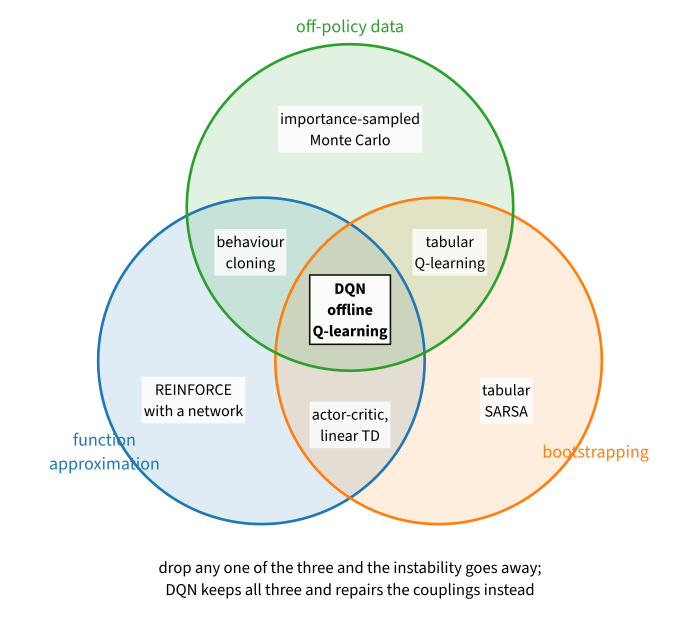
The three ingredients are function approximation, bootstrapping, and off-policy data. Figure Figure 15.4.1 locates familiar algorithms by which ingredients they use. Removing function approximation gives tabular Q-learning, which converges under the conditions of Section 14.4. Removing bootstrapping gives neural REINFORCE with Monte Carlo targets and an unbiased policy gradient. Removing off-policy data gives methods such as SARSA and on-policy actor–critic.
These comparisons do not imply that every method using only two ingredients converges. Nonlinear on-policy temporal-difference learning can also diverge, and positive results require assumptions about step sizes, coverage, and representation. The term deadly triad refers to the particularly difficult combination of all three ingredients (Sutton and Barto 2018; Hasselt et al. 2018).
Baird’s counterexample isolates this combination in a seven-state linear problem (Baird 1995). Every reward is zero, so the true value function is zero and can be represented exactly by \(w=0\). The experiment uses expected temporal-difference updates, eliminating sampling noise, but weights the seven states according to an off-policy distribution while evaluating a policy that always transitions to state seven:
w = np.ones(8)                             # eight weights for seven states
w[6] = 10.0                                # the classic starting point
Phi = np.zeros((7, 8))                     # linear values v = Phi w
Phi[:6, :6], Phi[:6, 7] = 2 * np.eye(6), 1.0   # v(i) = 2 w_i + w_8
Phi[6, 6], Phi[6, 7] = 1.0, 2.0                # v(7) = w_7 + 2 w_8
sup = []
for _ in range(1000):
    v = Phi @ w                            # every reward is 0
    delta = gamma * v[6] - v               # the next state is always state 7
    w += 0.01 * (delta[:, None] * Phi).mean(0)   # uniform state weighting
    sup.append(np.abs(w).max())
print(f'sup norm of w after 0, 500, 1000 sweeps: 10, {sup[499]:.0f}, '
      f'{sup[-1]:.0f}')
print(f'the value the weights claim for state 7: {(Phi @ w)[6]:.0f}, '
      f'true value 0')
d2l.plot(np.arange(1, 1001), sup, 'sweeps over all seven states',
         'sup norm of w', yscale='log')
sup norm of w after 0, 500, 1000 sweeps: 10, 77, 335
the value the weights claim for state 7: 677, true value 0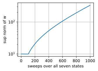
w = np.ones(8)                             # eight weights for seven states
w[6] = 10.0                                # the classic starting point
Phi = np.zeros((7, 8))                     # linear values v = Phi w
Phi[:6, :6], Phi[:6, 7] = 2 * np.eye(6), 1.0   # v(i) = 2 w_i + w_8
Phi[6, 6], Phi[6, 7] = 1.0, 2.0                # v(7) = w_7 + 2 w_8
sup = []
for _ in range(1000):
    v = Phi @ w                            # every reward is 0
    delta = gamma * v[6] - v               # the next state is always state 7
    w += 0.01 * (delta[:, None] * Phi).mean(0)   # uniform state weighting
    sup.append(np.abs(w).max())
print(f'sup norm of w after 0, 500, 1000 sweeps: 10, {sup[499]:.0f}, '
      f'{sup[-1]:.0f}')
print(f'the value the weights claim for state 7: {(Phi @ w)[6]:.0f}, '
      f'true value 0')
d2l.plot(np.arange(1, 1001), sup, 'sweeps over all seven states',
         'sup norm of w', yscale='log')
sup norm of w after 0, 500, 1000 sweeps: 10, 77, 335
the value the weights claim for state 7: 677, true value 0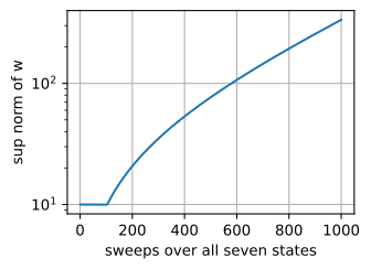
The weights grow approximately exponentially: after a thousand sweeps, their sup norm has increased from \(10\) to \(335\), and the estimated value of state 7 is \(677\) although its true value is zero. This deterministic expected-update calculation has no sampling error, and reducing the step size slows but does not remove the divergence. The cause is the composition of projection under the off-policy weighting with a bootstrapped backup (Tsitsiklis and Van Roy 1997). Reweighting the updates by the evaluated policy’s visitation distribution converges in this example (exercise 7).
Replay and target networks do not remove an element of the triad. They reduce temporal correlation and slow target changes, which often improves empirical stability but does not restore a general convergence guarantee.
15.4.2 Replay and Target Networks
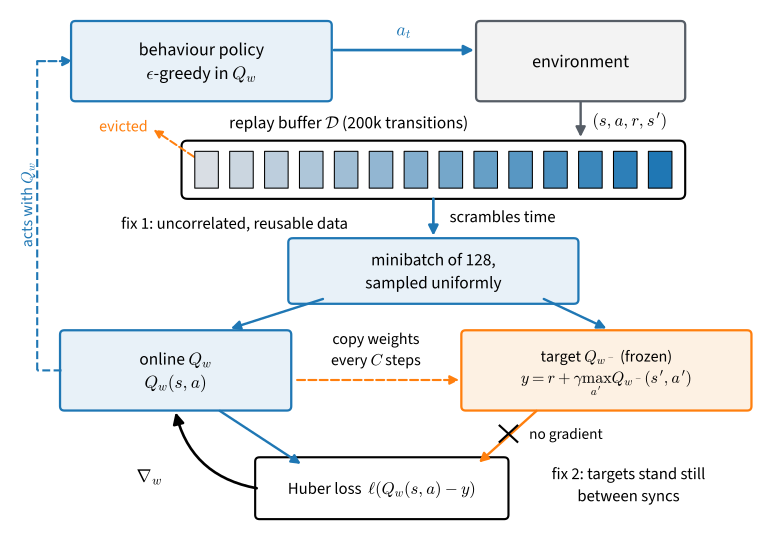
Figure 15.4.2 draws the whole machine; the two subsections that follow walk its two ideas.
15.4.2.1 Experience Replay and Off-Policy Updates
The standard remedy for temporal correlation is an experience replay buffer (Lin 1992). Transitions are stored in a finite array, and training minibatches are sampled uniformly from that array. A minibatch therefore combines transitions collected at different times, and each transition may be used in several updates. This is valid for Q-learning because the target for \((s,a,r,s')\) does not depend on the policy that selected \(a\). The same property will be central to the distinction between on-policy and off-policy learning in Section 15.6.
class ReplayBuffer:
    """A ring of transitions in preallocated numpy; sample() returns a Batch."""
    def __init__(self, capacity, obs_dim):
        self.obs = np.zeros((capacity, obs_dim), np.float32)
        self.act = np.zeros(capacity, np.int64)
        self.rew = np.zeros(capacity, np.float32)
        self.next_obs = np.zeros((capacity, obs_dim), np.float32)
        self.term = np.zeros(capacity, np.float32)
        self.capacity, self.size, self.ptr = capacity, 0, 0

    def add(self, obs, act, rew, next_obs, term):
        i = self.ptr
        self.obs[i], self.act[i], self.rew[i] = obs, act, rew
        self.next_obs[i], self.term[i] = next_obs, term
        self.ptr, self.size = (i + 1) % self.capacity, min(self.size + 1,
                                                           self.capacity)

    def __len__(self):
        return self.size

    def sample(self, batch_size, rng):
        i = rng.integers(self.size, size=batch_size)
        return d2l.Batch(self.obs[i], self.act[i], self.rew[i],
                         self.next_obs[i], self.term[i],
                         np.array([batch_size]))
class ReplayBuffer:
"""A ring of transitions in preallocated numpy; sample() returns a Batch."""
def __init__(self, capacity, obs_dim):
self.obs = np.zeros((capacity, obs_dim), np.float32)
self.act = np.zeros(capacity, np.int64)
self.rew = np.zeros(capacity, np.float32)
self.next_obs = np.zeros((capacity, obs_dim), np.float32)
self.term = np.zeros(capacity, np.float32)
self.capacity, self.size, self.ptr = capacity, 0, 0
def add(self, obs, act, rew, next_obs, term):
i = self.ptr
self.obs[i], self.act[i], self.rew[i] = obs, act, rew
self.next_obs[i], self.term[i] = next_obs, term
self.ptr, self.size = (i + 1) % self.capacity, min(self.size + 1,
self.capacity)
def __len__(self):
return self.size
def sample(self, batch_size, rng):
i = rng.integers(self.size, size=batch_size)
return d2l.Batch(self.obs[i], self.act[i], self.rew[i],
self.next_obs[i], self.term[i],
np.array([batch_size]))Two details of the container matter. Its capacity is \(200{,}000\) transitions, larger than the \(50{,}000\)-step training budget, so no transition is evicted in these experiments; exercise 4 studies a smaller buffer. In addition, sample returns a Batch without episode structure. Consequently, reward_to_go and gae are not defined for such a batch, whereas td_target requires only individual transitions. This is why replay combines naturally with one-step bootstrapping. The target below is the same batch.td_target used by the actor-critic critic.
15.4.2.2 The Target Network
The repair for moving targets is the target network (Mnih et al. 2015): a frozen copy \(Q_{w^-}\) of the online network computes every bootstrap,
\[y = r + \gamma\, \big(1 - \mathbf{1}(s' \textrm{ terminal})\big) \max_{a'} Q_{w^-}(s', a'), \tag{15.4.2}\]
and synchronize the copy with the online weights, \(w^-\leftarrow w\), every \(C\) steps, here every 250. Between synchronizations, the target is fixed and the online network solves an ordinary regression problem. The feedback from predictions to targets now occurs once per synchronization rather than once per gradient step. The actor–critic method in Section 15.1 updates its target from the newest critic because each batch contains fresh on-policy data. Replay removes that freshness, so DQN instead accepts stale targets to reduce the rate at which the regression problem changes.
The regression update uses two distinct controls. The Huber loss is quadratic near zero and linear for large residuals, so it bounds the derivative of the loss with respect to the prediction. The parameter gradient also contains \(\nabla_w Q_w(s,a)\), which the Huber loss does not bound. Global norm clipping therefore limits the complete parameter update, including the large simultaneous residual changes that may follow a target-network synchronization.
def q_values(qnet, obs):
    """The acting forward: numpy in, numpy out, no gradient recorded."""
    with torch.inference_mode():
        return qnet(torch.as_tensor(obs)).numpy()

def fit_q(qnet, opt, batch, y):
    """One clipped Huber regression step of Q_w(s, a) toward the fixed y."""
    pred = qnet(torch.as_tensor(batch.obs)).gather(
        -1, torch.as_tensor(batch.act)[:, None]).squeeze(-1)
    loss = nn.functional.huber_loss(pred, torch.as_tensor(y))
    opt.zero_grad()
    loss.backward()
    nn.utils.clip_grad_norm_(qnet.parameters(), grad_clip)
    opt.step()

def q_step(qnet, target, opt, batch):
    """The DQN update: the critic's own td_target, bootstrapped by the copy."""
    fit_q(qnet, opt, batch, batch.td_target(
        lambda s: q_values(target, s).max(-1), gamma))
def fit_q(qnet, opt, obs, act, y):
"""One Huber regression step of Q_w(s, a) toward the fixed y; traced
inside the jitted steps, with the norm clip in the optimizer chain."""
_, grads = nnx.value_and_grad(lambda q: optax.huber_loss(
jnp.take_along_axis(q(obs), act[:, None], -1).squeeze(-1),
y).mean())(qnet)
opt.update(qnet, grads)
@nnx.jit
def q_step(qnet, target, opt, obs, act, rew, next_obs, term):
"""The DQN update. The target line is Batch.td_target's expression,
computed inside the compiled step (:numref:`sec_compilation`)."""
fit_q(qnet, opt, obs, act,
rew + gamma * (1 - term) * target(next_obs).max(-1))
_q_forward, _cached = nnx.jit(lambda net, obs: net(obs)), {}
def q_values(qnet, obs):
"""The acting forward: compiled once, module traversal cached, because
the loop below calls it once per environment step."""
if id(qnet) not in _cached:
_cached[id(qnet)] = nnx.cached_partial(_q_forward, qnet)
return np.asarray(_cached[id(qnet)](jnp.asarray(obs)))One hairline detail separates the two tabs. The pytorch update literally calls batch.td_target, the structural thesis in a single line; the jax update runs a couple of hundred thousand times and is compiled, and a compiled function cannot call back into a numpy method, so it computes the same expression inline (Section 13.3). The next cell certifies that “the same expression” is not a figure of speech, on a buffer filled by a random policy through the rollout helper both chapters share:
rng, env = np.random.default_rng(0), gym.make('CartPole-v1')
env.reset(seed=0)
data = d2l.rollout(env, lambda s, r: int(r.integers(2)), 20, rng)
buffer = ReplayBuffer(buffer_size, 4)
for i in range(len(data)):
    buffer.add(data.obs[i], data.act[i], data.rew[i],
               data.next_obs[i], data.term[i])
b = buffer.sample(batch_size, rng)
torch.manual_seed(0)
tnet = make_qnet()
with torch.inference_mode():
    y = (torch.as_tensor(b.rew) + gamma * (1 - torch.as_tensor(b.term))
         * tnet(torch.as_tensor(b.next_obs)).max(-1).values).numpy()
print(np.allclose(y, b.td_target(lambda s: q_values(tnet, s).max(-1), gamma)))Truerng, env = np.random.default_rng(0), gym.make('CartPole-v1')
env.reset(seed=0)
data = d2l.rollout(env, lambda s, r: int(r.integers(2)), 20, rng)
buffer = ReplayBuffer(buffer_size, 4)
for i in range(len(data)):
buffer.add(data.obs[i], data.act[i], data.rew[i],
data.next_obs[i], data.term[i])
b = buffer.sample(batch_size, rng)
tnet = make_qnet(nnx.Rngs(0))
y = np.asarray(jnp.asarray(b.rew) + gamma * (1 - jnp.asarray(b.term))
* tnet(jnp.asarray(b.next_obs)).max(-1))
print(np.allclose(y, b.td_target(lambda s: q_values(tnet, s).max(-1), gamma)))TrueNow the training loop, and it is short because everything it needs already exists: epsilon_greedy and linear_schedule from Section 14.4, the buffer and step above. One switch controls the experiment of this section. With use_target=True the copy refreshes every sync_every steps; with use_target=False it refreshes every step, which makes the copy the online network in all but name, the naive recipe with no target network at all. The generator yields, at every episode’s end, the step count, the episode’s return, and one diagnostic we will need later: the network’s value estimate \(\max_a Q_w(s_0, a)\) at the centered start state \(s_0 = \mathbf{0}\).
def train_dqn(seed, qnet, use_target=True, step=None):
    """DQN on CartPole; yields (env step, episode return, max_a Q(s0, a))."""
    step = q_step if step is None else step
    rng, env = np.random.default_rng(seed), gym.make('CartPole-v1')
    target = make_qnet()
    target.load_state_dict(qnet.state_dict())
    opt = torch.optim.Adam(qnet.parameters(), lr=lr)
    buffer, s0 = ReplayBuffer(buffer_size, 4), np.zeros(4, np.float32)
    obs, ep_return = env.reset(seed=seed)[0], 0.0
    sync = sync_every if use_target else 1
    for t in range(1, num_env_steps + 1):
        a = d2l.epsilon_greedy(q_values(qnet, obs), epsilon(t), rng)
        next_obs, rew, terminated, truncated, _ = env.step(a)
        buffer.add(obs, a, rew, next_obs, float(terminated))
        obs, ep_return = next_obs, ep_return + rew
        if terminated or truncated:
            yield t, ep_return, q_values(qnet, s0).max()
            obs, ep_return = env.reset()[0], 0.0
        if len(buffer) >= warmup and t % train_freq == 0:
            step(qnet, target, opt, buffer.sample(batch_size, rng))
        if t % sync == 0:
            target.load_state_dict(qnet.state_dict())
def train_dqn(seed, qnet, use_target=True, step=None):
"""DQN on CartPole; yields (env step, episode return, max_a Q(s0, a)).
The jitted step's module traversal is cached once per run."""
step = q_step if step is None else step
rng, env = np.random.default_rng(seed), gym.make('CartPole-v1')
target = nnx.clone(qnet)
opt = nnx.Optimizer(qnet, optax.chain(
optax.clip_by_global_norm(grad_clip), optax.adam(lr)), wrt=nnx.Param)
step_fn = nnx.cached_partial(step, qnet, target, opt)
buffer, s0 = ReplayBuffer(buffer_size, 4), np.zeros(4, np.float32)
obs, ep_return = env.reset(seed=seed)[0], 0.0
sync = sync_every if use_target else 1
for t in range(1, num_env_steps + 1):
a = d2l.epsilon_greedy(q_values(qnet, obs), epsilon(t), rng)
next_obs, rew, terminated, truncated, _ = env.step(a)
buffer.add(obs, a, rew, next_obs, float(terminated))
obs, ep_return = next_obs, ep_return + rew
if terminated or truncated:
yield t, ep_return, q_values(qnet, s0).max()
obs, ep_return = env.reset()[0], 0.0
if len(buffer) >= warmup and t % train_freq == 0:
b = buffer.sample(batch_size, rng)
step_fn(jnp.asarray(b.obs), jnp.asarray(b.act),
jnp.asarray(b.rew), jnp.asarray(b.next_obs),
jnp.asarray(b.term))
if t % sync == 0:
nnx.update(target, nnx.state(qnet, nnx.Param))Note what the buffer stores: terminated, never truncated. A CartPole episode cut off at 500 steps ends in a state with a future, and Section 14.4 established that masking the bootstrap there teaches the network that surviving is worthless; exercise 2 traces exactly what would go wrong.
15.4.2.3 Ablating the Target Network
Three seeds per arm, everything identical except the switch. The networks are caller-owned, as in Section 15.1, so later cells can audit the trained agents:
if tab.selected('pytorch'):
    def new_qnet(seed):
        torch.manual_seed(seed)
        return make_qnet()
if tab.selected('jax'):
    def new_qnet(seed):
        return make_qnet(nnx.Rngs(seed))

arms = ('DQN', 'no target network')
qnets = {arm: [new_qnet(seed) for seed in range(num_seeds)] for arm in arms}
runs = {arm: [list(train_dqn(seed, qnets[arm][seed],
                             use_target=arm == 'DQN'))
              for seed in range(num_seeds)] for arm in arms}
if tab.selected('pytorch'):
def new_qnet(seed):
torch.manual_seed(seed)
return make_qnet()
if tab.selected('jax'):
def new_qnet(seed):
return make_qnet(nnx.Rngs(seed))
arms = ('DQN', 'no target network')
qnets = {arm: [new_qnet(seed) for seed in range(num_seeds)] for arm in arms}
runs = {arm: [list(train_dqn(seed, qnets[arm][seed],
use_target=arm == 'DQN'))
for seed in range(num_seeds)] for arm in arms}Each run yields one tuple per episode, and seeds finish different numbers of episodes, so the right x axis is the one the budget is written in. We resample every curve onto a common grid of environment steps and plot the seed bands:
grid = np.arange(1, num_env_steps // 1000 + 1) * 1000

def on_grid(arm, col):
    """Resample each seed's per-episode series onto the env-step grid."""
    return np.stack([np.interp(grid, np.asarray(r)[:, 0], np.asarray(r)[:, col])
                     for r in runs[arm]])

d2l.plot_curves({arm: on_grid(arm, 1) for arm in runs},
                xlabel='thousand environment steps',
                ylabel='return of the behavior policy', smooth=5,
                reference=500)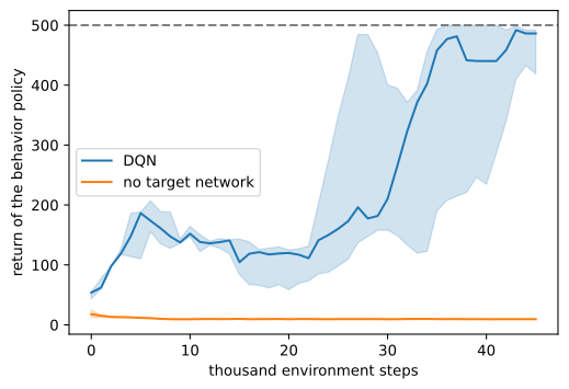
grid = np.arange(1, num_env_steps // 1000 + 1) * 1000

def on_grid(arm, col):
    """Resample each seed's per-episode series onto the env-step grid."""
    return np.stack([np.interp(grid, np.asarray(r)[:, 0], np.asarray(r)[:, col])
                     for r in runs[arm]])

d2l.plot_curves({arm: on_grid(arm, 1) for arm in runs},
                xlabel='thousand environment steps',
                ylabel='return of the behavior policy', smooth=5,
                reference=500)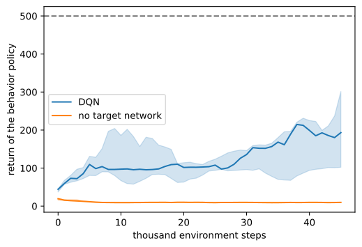
The two variants differ only in whether the bootstrap uses a target network. With a target network, every seed improves from the random policy’s return of about 20, although learning remains variable and no seed remains at the maximum return of 500. The behavior-policy curve cannot reach 500 consistently because the final exploration rate is \(\epsilon=0.05\), which forces a random action on approximately one step in twenty. Without a target network, returns improve briefly and then collapse for every seed in both framework implementations. The online network then supplies its own changing targets, and the poor greedy policy collects data that reinforces the same estimates. The separate greedy evaluation below removes exploratory actions from the comparison.
Because the return keeps falling off its peaks and climbing back, the summary statistic you choose matters more than it should, and the next cell computes the candidates rather than asserting them. For each seed we take every trailing 20-episode average the run contains, and report the best one, the final one, and the one the run would have reported had we stopped it fifty episodes earlier:
def windows(returns, k=20):
    """All trailing k-episode averages of a run, in order."""
    return np.convolve(returns, np.ones(k) / k, 'valid')

for arm in runs:
    w = [windows(np.asarray(r)[:, 1]) for r in runs[arm]]
    best = np.array([x.max() for x in w])
    final = np.array([x[-1] for x in w])
    early = np.array([x[-51] for x in w])
    print(f'{arm:>18}: best 20-episode window per seed {np.round(best)}\n'
          f'{"":>18}  final window {np.round(final)} '
          f'(spread {np.ptp(final):.0f})\n'
          f'{"":>18}  fifty episodes earlier {np.round(early)}')
DQN: best 20-episode window per seed [500. 348. 457.]
final window [496. 348. 431.] (spread 148)
fifty episodes earlier [163. 99. 203.]
no target network: best 20-episode window per seed [30. 27. 25.]
final window [9. 9. 9.] (spread 0)
fifty episodes earlier [10. 10. 10.]def windows(returns, k=20):
"""All trailing k-episode averages of a run, in order."""
return np.convolve(returns, np.ones(k) / k, 'valid')
for arm in runs:
w = [windows(np.asarray(r)[:, 1]) for r in runs[arm]]
best = np.array([x.max() for x in w])
final = np.array([x[-1] for x in w])
early = np.array([x[-51] for x in w])
print(f'{arm:>18}: best 20-episode window per seed {np.round(best)}\n'
f'{"":>18} final window {np.round(final)} '
f'(spread {np.ptp(final):.0f})\n'
f'{"":>18} fifty episodes earlier {np.round(early)}') DQN: best 20-episode window per seed [256. 104. 233.]
final window [163. 98. 233.] (spread 136)
fifty episodes earlier [162. 94. 157.]
no target network: best 20-episode window per seed [27. 25. 26.]
final window [ 9. 10. 10.] (spread 0)
fifty episodes earlier [10. 10. 10.]The final-window return varies by more than one hundred points across seeds, and the value fifty episodes earlier differs again. It therefore describes the state of each training run at the stopping time rather than a stable endpoint. Selecting the best window after observing the entire curve introduces optimistic selection bias; reporting its seed spread does not remove that bias.
For evaluation, we predeclare a budget of \(50{,}000\) environment steps and then evaluate the resulting policy separately. This separates the policy from the exploration noise in the training return and avoids choosing a stopping point after inspecting the curves.
The behavior return combines policy quality with the effect of \(\epsilon\)-greedy exploration. After the fixed training budget, we therefore evaluate the greedy policy separately with \(\epsilon=0\):
env = gym.make('CartPole-v1')
for arm in arms:
    for seed in range(num_seeds):
        env.reset(seed=100 + seed)
        qnet = qnets[arm][seed]
        score = d2l.evaluate(env, lambda s, r: int(q_values(qnet, s).argmax()),
                             num_episodes=100)
        print(f'{arm:>18}, seed {seed}: greedy return over 100 episodes '
              f'{score:.0f}')
DQN, seed 0: greedy return over 100 episodes 500
DQN, seed 1: greedy return over 100 episodes 93
DQN, seed 2: greedy return over 100 episodes 500
no target network, seed 0: greedy return over 100 episodes 10
no target network, seed 1: greedy return over 100 episodes 9
no target network, seed 2: greedy return over 100 episodes 9env = gym.make('CartPole-v1')
for arm in arms:
for seed in range(num_seeds):
env.reset(seed=100 + seed)
qnet = qnets[arm][seed]
score = d2l.evaluate(env, lambda s, r: int(q_values(qnet, s).argmax()),
num_episodes=100)
print(f'{arm:>18}, seed {seed}: greedy return over 100 episodes '
f'{score:.0f}') DQN, seed 0: greedy return over 100 episodes 220
DQN, seed 1: greedy return over 100 episodes 152
DQN, seed 2: greedy return over 100 episodes 500
no target network, seed 0: greedy return over 100 episodes 10
no target network, seed 1: greedy return over 100 episodes 9
no target network, seed 2: greedy return over 100 episodes 9Without exploratory actions, some seeds achieve the maximum return of 500, while others score far below their recent behavior returns. The final greedy policy is a single snapshot of an oscillatory training process, so evaluation depends on the point at which training stops. Across frameworks and seeds, the greedy returns range from roughly 90 to 500. Every run without a target network fails almost immediately.
To distinguish value instability from policy instability, the training loop records \(\max_a Q_w(s_0,a)\) at the centered start state. The code masks bootstrapping only on terminated; it continues to bootstrap across the 500-step time limit, and the state contains no time coordinate. It therefore learns the continuing-task value in which the time limit ends data collection but not the underlying process.
In this formulation, a policy that balances the pole indefinitely has value \(1/(1-\gamma)=100\) from the start. The dashed line marks this ceiling:
ceiling = 1 / (1 - gamma)
d2l.plot_curves({'DQN': on_grid('DQN', 2)},
                xlabel='thousand environment steps',
                ylabel='value estimate at the start state',
                reference=ceiling)
print(f'continuing-task ceiling: {ceiling:.0f}; the no-target arm ends at ' +
      ', '.join(f'{np.asarray(r)[-1, 2]:.0e}' for r in
                runs['no target network']))
continuing-task ceiling: 100; the no-target arm ends at 1e+08, 1e+08, 1e+08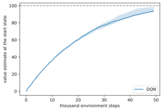
ceiling = 1 / (1 - gamma)
d2l.plot_curves({'DQN': on_grid('DQN', 2)},
                xlabel='thousand environment steps',
                ylabel='value estimate at the start state',
                reference=ceiling)
print(f'continuing-task ceiling: {ceiling:.0f}; the no-target arm ends at ' +
      ', '.join(f'{np.asarray(r)[-1, 2]:.0e}' for r in
                runs['no target network']))
continuing-task ceiling: 100; the no-target arm ends at 2e+08, 2e+08, 2e+08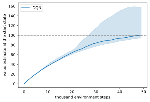
For DQN, the recorded start-state estimate remains within tens of points of the continuing-task ceiling across frameworks and seeds. The corresponding return curves still oscillate because small changes in action values can change the greedy action and produce a substantially different policy. This trace concerns only \(s_0\) and does not certify that every Q-value is stable or accurate.
The scale nevertheless separates the two ablations. DQN ends near \(10^2\), whereas the version without a target network exceeds \(10^8\). The latter clearly diverges. Some DQN seeds settle above the ceiling of 100. Since no policy can exceed that value under the objective implemented here, those estimates demonstrate overestimation.
The next experiment isolates the maximization bias that produces this effect.
15.4.3 Overestimation
15.4.3.1 Measuring the Maximization Bias
The target Equation 15.4.2 maximizes estimated action values. For noisy estimates, \(E[\max_{a'}\hat{Q}(s',a')]\geq\max_{a'}E[\hat{Q}(s',a')]\), with strict inequality when noise can change the maximizing action. Section 14.4 demonstrated this bias in a table, and Section 15.3 showed that the hard maximum is the \(\beta\to0\) limit of the soft backup. Function approximation can feed the resulting bias back into subsequent targets (Thrun and Schwartz 1993).
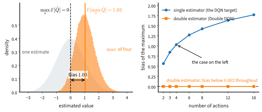
The following simulation gives four actions the same true value of zero and adds independent unit noise to each estimate. The single estimator selects and evaluates an action with the same noisy values. The double estimator selects with one set of noisy values and evaluates with an independent set (Hasselt 2010):
rng = np.random.default_rng(0)
est = rng.standard_normal((100_000, 4))     # four values, all truly zero
second = rng.standard_normal((100_000, 4))  # an independent second estimate
sel = est.argmax(1)
print(f'single estimator, E[max of the estimates]: {est.max(1).mean():.3f}')
print(f'select with one, evaluate with the other: '
      f'{second[np.arange(100_000), sel].mean():+.3f}')
single estimator, E[max of the estimates]: 1.031
select with one, evaluate with the other: -0.006rng = np.random.default_rng(0)
est = rng.standard_normal((100_000, 4)) # four values, all truly zero
second = rng.standard_normal((100_000, 4)) # an independent second estimate
sel = est.argmax(1)
print(f'single estimator, E[max of the estimates]: {est.max(1).mean():.3f}')
print(f'select with one, evaluate with the other: '
f'{second[np.arange(100_000), sel].mean():+.3f}')single estimator, E[max of the estimates]: 1.031
select with one, evaluate with the other: -0.006The maximum of four unit-noise estimates has about one unit of upward bias. With independent selection and evaluation estimates, the evaluator’s noise has zero conditional mean for the selected action, and the measured bias is near zero. Figure 15.4.3 shows that the single-estimator bias grows with the number of actions while the independent double estimator remains near zero. In DQN, shared parameters and bootstrapping can propagate this bias to other states; a fixed offline dataset also removes the corrective effect of new interaction (Section 15.6).
15.4.3.2 Double DQN
The double estimator requires two value estimates, and DQN already maintains an online network and a target network. Double DQN uses the online network to select the action and the target network to evaluate it (Van Hasselt et al. 2016):
\[y = r + \gamma\, \big(1 - \mathbf{1}(s' \textrm{ terminal})\big)\ Q_{w^-}\big(s',\ \underset{a'}{\mathrm{argmax}}\ Q_w(s', a')\big). \tag{15.4.3}\]
An action selected by an overestimate in the online network is therefore not evaluated by that same output. The target copy is correlated with the online network, so Double DQN only approximates the independent double estimator analyzed above. It reuses the two forward passes already required by DQN; the change to q_step is three lines:
def q_step_double(qnet, target, opt, batch):
    """q_step with selection split from evaluation, eq_double_dqn."""
    sel = q_values(qnet, batch.next_obs).argmax(-1)
    fit_q(qnet, opt, batch, batch.td_target(
        lambda s: q_values(target, s)[np.arange(len(s)), sel], gamma))
@nnx.jit
def q_step_double(qnet, target, opt, obs, act, rew, next_obs, term):
"""q_step with selection split from evaluation, eq_double_dqn."""
sel = qnet(next_obs).argmax(-1)
fit_q(qnet, opt, obs, act, rew + gamma * (1 - term) * jnp.take_along_axis(
target(next_obs), sel[:, None], -1).squeeze(-1))The training loop changes only the update function; data collection, replay, target synchronization, and evaluation remain fixed. We use the same logged diagnostic for the comparison:
qnets['Double DQN'] = [new_qnet(seed) for seed in range(num_seeds)]
runs['Double DQN'] = [list(train_dqn(seed, qnets['Double DQN'][seed],
                                     step=q_step_double))
for seed in range(num_seeds)]qnets['Double DQN'] = [new_qnet(seed) for seed in range(num_seeds)]
runs['Double DQN'] = [list(train_dqn(seed, qnets['Double DQN'][seed],
step=q_step_double))
for seed in range(num_seeds)]d2l.plot_curves({arm: on_grid(arm, 2) for arm in ('DQN', 'Double DQN')},
xlabel='thousand environment steps',
ylabel='value estimate at the start state',
reference=ceiling)
for arm in ('DQN', 'Double DQN'):
print(f'{arm:>10}: final value estimate at s0, per seed: '
f'{np.round([np.asarray(r)[-1, 2] for r in runs[arm]], 1)}') DQN: final value estimate at s0, per seed: [93.8 98.3 93. ]
Double DQN: final value estimate at s0, per seed: [92.6 95.1 91. ]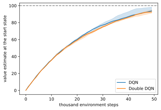
d2l.plot_curves({arm: on_grid(arm, 2) for arm in ('DQN', 'Double DQN')},
                xlabel='thousand environment steps',
                ylabel='value estimate at the start state',
                reference=ceiling)
for arm in ('DQN', 'Double DQN'):
    print(f'{arm:>10}: final value estimate at s0, per seed: '
          f'{np.round([np.asarray(r)[-1, 2] for r in runs[arm]], 1)}')
DQN: final value estimate at s0, per seed: [100.3 157. 94.4]
Double DQN: final value estimate at s0, per seed: [ 97.1 109.2 92.7]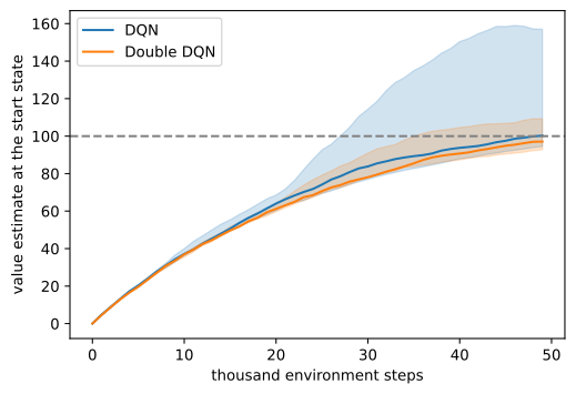
The Double DQN estimates usually end a few points below the DQN estimates, with the largest reductions in seeds that had moved furthest above the ceiling. Their seed bands overlap during most of training. CartPole has only two actions, and Figure 15.4.3 shows that maximization bias grows with the number of actions. The effect is therefore expected to be small here.
On Atari, with as many as eighteen actions, Double DQN changes scores substantially (Van Hasselt et al. 2016). The same distinction becomes important in offline learning, where inflated actions cannot be corrected by new interaction (Section 15.6). At this CartPole budget, any difference in return remains within variation across seeds.
15.4.4 The DQN Lineage
15.4.4.1 Extensions and Successors
Several later methods modify individual components of DQN. An \(n\)-step target uses several observed rewards before bootstrapping, as developed in Section 15.1. Prioritized replay samples transitions according to their temporal-difference error rather than uniformly (Schaul et al. 2016); its advantage decreases as replay buffers become larger and more diverse. A dueling network represents \(Q\) as a state value plus action advantages (Wang et al. 2016).
Distributional methods estimate the return distribution rather than only its mean (Bellemare et al. 2017). In tabular and linear settings, their expected update for the mean coincides with the ordinary update, so their empirical benefit depends on the interaction with nonlinear function approximation. Rainbow combines six extensions and reports an ablation of their individual contributions (Hessel et al. 2018).
PQN provides a contrasting design: with LayerNorm and batches collected from parallel environments, deep Q-learning can train without a replay buffer or target network (Gallici et al. 2025). Replay and target networks are therefore one solution to correlated data and moving targets, not necessary components of every stable deep Q-learning system.
15.4.4.2 DQN in Modern Practice
Vanilla DQN is mainly useful here as a simple setting in which to study two problems of deep value learning: moving bootstrap targets and maximization bias. It also establishes how a learner can use transitions collected by a different policy. Since the policy requires an argmax over actions, the basic method is restricted to discrete action spaces; actor-based methods extend related ideas to continuous control. Section 15.6 considers the limiting case in which all learning uses a fixed dataset and no further interaction is allowed.
15.4.5 Summary
With function approximation, bootstrapping, and off-policy data, Q-learning can diverge even when the value class contains the correct solution. Experience replay reduces temporal correlation and reuses transitions, while a target network holds bootstrap targets fixed between updates. These mechanisms improve stability but do not restore the tabular convergence theorem. DQN also inherits maximization bias. Double DQN reduces this bias by selecting an action with the online network and evaluating it with the target network.
Experimental scope. Baird’s counterexample and the synthetic maximization-bias calculation are deterministic. The CartPole ablation uses three seeds per method and framework for \(50{,}000\) environment steps. Every run without a target network diverges beyond \(10^8\) in value, while the target-network runs learn but remain variable. Fixed-budget greedy evaluation is reported separately from exploratory training return. At two actions, the effect of Double DQN on return is smaller than the variation across runs.
15.4.6 Exercises
- [conceptual] What survives the scramble. A batch sampled from
ReplayBuffercarries a fake episode boundary. For each oftd_target,reward_to_go, andgae, state whether its value on such a batch is meaningful, and connect the pattern to the on-policy/off-policy split: why is the estimator that survives the scramble exactly the one whose target ignores the collector? - [conceptual] Terminated, not done. The buffer stores
float(terminated)and nevertruncated. Recalling Section 14.4’s masking discussion, describe precisely what the targets would teach the network about long CartPole episodes ifdonewere stored instead, and why the damage would grow as the policy improves. - [short-code] The sync period. Rerun the target arm with
sync_everyin \(\{50, 250, 2500\}\), one seed each. Distinguish two failure directions: does the bad end merely slow learning, or does it cap what the run reaches within the budget? Report fixed-budget greedy evaluations, with the best and final windows beside them as descriptions of the curve, and say why the distinction matters here of all places. - [short-code] Shrink the buffer. Set the capacity to 500 transitions and retrain one seed. Which of the two couplings does this reintroduce, what do the return curve and the \(\max_a Q_w(s_0, a)\) trace look like, and why does the failure wait until the policy is good before it arrives?
- [short-code] Best against final, at scale. Using only curves already logged by this section’s cells and exercise 3’s runs, no new training, collect the best-window and final-window statistics across every seed and arm. Which spread is a property of the algorithm and which is mostly a property of when you stopped looking, and why does a predeclared fixed-budget evaluation belong in a paper where neither window does?
- [short-code] Port it. Move the section’s code to
LunarLander-v3. List every line that changes and every line that does not, then explain why the step budget is the one number you should expect to raise substantially. (Running the port to a strong policy takes roughly ten times this section’s budget; the listing question is answerable without running at all.) - [extended] Baird, with a target network. Add a target network to the Baird cell: compute every \(\delta\) from a frozen copy of \(w\), synced every \(k\) sweeps, for \(k \in \{10, 100\}\). Does the iteration now converge, diverge more slowly, or diverge the same? Which corner of the triad did the target network actually remove, and what does the answer say about what DQN’s second repair can and cannot buy?