%matplotlib inline
from d2l import torch as d2l
import numpy as onp
import torch27.3 Maximum Likelihood
Many standard machine-learning losses arise from probabilistic models. Maximizing the probability of the observed data gives the maximum likelihood principle. Taking logarithms yields a negative log-likelihood; for common models this objective becomes cross-entropy or mean squared error. This section derives these relationships and then studies consistency, asymptotic normality, and Fisher information. Adding a prior gives MAP estimation and, in the Gaussian case, \(L_2\) regularization. For latent-variable models, the evidence lower bound and expectation–maximization replace a likelihood that is difficult to optimize directly. A coin-flip example provides a calculation that can be checked in closed form.
%matplotlib inline
from d2l import tensorflow as d2l
import numpy as onp
import tensorflow as tf%matplotlib inline
from d2l import jax as d2l
import jax
from jax import numpy as jnp
import numpy as onp%matplotlib inline
from d2l import mxnet as d2l
from mxnet import autograd, np, npx
import numpy as onp
npx.set_np()27.3.1 The Maximum Likelihood Principle
Suppose we have a model with parameters \(\boldsymbol{\theta}\) and observed data \(X\). The likelihood is the model probability or density of the observed data, viewed as a function of the parameter:
\[ L(\boldsymbol{\theta};X)=P(X\mid\boldsymbol{\theta}). \]
Maximum likelihood is the direct rule
\[ \hat{\boldsymbol{\theta}}_{\textrm{MLE}} = \mathop{\mathrm{argmax}}_{\boldsymbol{\theta}} P(X \mid \boldsymbol{\theta}). \tag{27.3.1}\]
No prior is part of this definition. MLE asks which member of the chosen model family fits the observations best; it does not assign probabilities to the parameters themselves. Later, Section 27.3.4 introduces the distinct maximum a posteriori rule \(\operatorname*{argmax}_{\boldsymbol{\theta}}P(\boldsymbol{\theta}\mid X)\), which multiplies the likelihood by a prior density. A prior that is constant in the chosen parameterization makes the two optimizers coincide, but “flat” is not invariant under nonlinear reparameterization and is not the foundation of maximum likelihood.
27.3.1.1 A Worked Example: The Coin
Take a single parameter \(\theta\), the probability of heads, so tails has probability \(1-\theta\). Because the flips are independent, their probabilities multiply: if \(X\) has \(n_H\) heads and \(n_T\) tails,
\[ P(X \mid \theta) = \theta^{n_H}(1-\theta)^{n_T}. \tag{27.3.2}\]
Suppose that \(13\) flips produce the sequence “HHHTHTTHHHHHT”, with \(n_H=9\) heads and \(n_T=4\) tails. The likelihood is then \(P(X \mid \theta)=\theta^9(1-\theta)^4\). The empirical fraction of heads, \(9/13\), is the natural estimate of the bias. Maximum likelihood derives this estimate from a general principle that also applies when the parameters cannot be estimated by inspection.
The likelihood is a function of \(\theta\) alone, so we can plot it and read off its peak.
import numpy as onp
theta = onp.arange(0, 1, 0.001)
p = theta**9 * (1 - theta)**4.

d2l.plot(theta, p, 'theta', 'likelihood')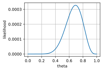
The curve peaks near the expected \(9/13 \approx 0.69\). To pin the maximum exactly we use calculus: at an interior maximum the derivative vanishes. Setting \(\frac{d}{d\theta}P(X\mid\theta)=0\),
\[ 0 = \frac{d}{d\theta}\,\theta^9(1-\theta)^4 = 9\theta^8(1-\theta)^4 - 4\theta^9(1-\theta)^3 = \theta^8(1-\theta)^3(9-13\theta). \]
The roots \(\theta=0\) and \(\theta=1\) assign probability zero to a sequence that contains both heads and tails, so they are minima. The remaining root is the maximum likelihood estimate,
\[ \hat\theta = \frac{9}{13}, \]
the observed fraction of heads. The same calculation on the general likelihood Equation 27.3.2 gives \(\hat\theta = n_H/(n_H+n_T)\): the MLE of a coin’s bias is the empirical frequency of heads.
27.3.1.2 The Negative Log-Likelihood
The closed-form trick above does not extend to a real model: with billions of parameters there is no polynomial to factor, and we optimize numerically instead. But the likelihood itself is unusable in floating point. With \(n\) independent data points it is a product of \(n\) probabilities,
\[ P(X\mid\boldsymbol{\theta}) = \prod_{i=1}^n p(x_i\mid\boldsymbol{\theta}), \]
each in \([0,1]\). A billion factors near \(1/2\) produce roughly \((1/2)^{10^9}\), underflowing to zero in any floating-point format long before we can differentiate it.
The logarithm rescues us, turning the product into a sum that stays in range:
\[ \log\!\big((1/2)^{10^9}\big) = 10^9 \cdot \log(1/2) \approx -6.93\times10^{8}, \]
which fits comfortably even in single precision. Since \(x \mapsto \log x\) is strictly increasing, it preserves the location of the maximum, so maximizing the likelihood is the same as maximizing the log-likelihood \(\log P(X\mid\boldsymbol{\theta})\). We use this exact reasoning for the naive Bayes classifier in Section 27.7. Finally, because we prefer to minimize losses, we flip the sign and define the negative log-likelihood (NLL):
\[ \ell(\boldsymbol{\theta}) = -\log P(X\mid\boldsymbol{\theta}) = -\sum_{i=1}^n \log p(x_i\mid\boldsymbol{\theta}). \tag{27.3.3}\]
For the coin this reads \(\ell(\theta) = -\big(n_H\log\theta + n_T\log(1-\theta)\big)\), which we can minimize by gradient descent even for billions of flips, no closed form required. The cell below does exactly this for almost nine million flips and confirms it recovers \(n_H/(n_H+n_T)\).
# Set up our data
n_H = 8675309
n_T = 256245

# Initialize our parameters
theta = torch.tensor(0.5, requires_grad=True)

# Perform gradient descent
lr = 1e-9
for iter in range(100):
    loss = -(n_H * torch.log(theta) + n_T * torch.log(1 - theta))
    loss.backward()
    with torch.no_grad():
        theta -= lr * theta.grad
    theta.grad.zero_()

# Check output
theta, n_H / (n_H + n_T)
(tensor(0.9713, requires_grad=True), 0.9713101437890875)# Set up our data
n_H = 8675309
n_T = 256245
# Initialize our parameters
theta = tf.Variable(tf.constant(0.5))
# Perform gradient descent
lr = 1e-9
for iter in range(100):
with tf.GradientTape() as t:
loss = -(n_H * tf.math.log(theta) + n_T * tf.math.log(1 - theta))
theta.assign_sub(lr * t.gradient(loss, theta))
# Check output
theta, n_H / (n_H + n_T)(<tf.Variable 'Variable:0' shape=() dtype=float32, numpy=0.9713100790977478>,
0.9713101437890875)# Set up our data
n_H = 8675309
n_T = 256245
# Initialize our parameters
theta = jnp.float32(0.5)
# Define loss function
def nll(theta):
return -(n_H * jnp.log(theta) + n_T * jnp.log(1 - theta))
grad_fn = jax.grad(nll)
# Perform gradient descent
lr = 1e-9
for iter in range(100):
theta = theta - lr * grad_fn(theta)
# Check output
theta, n_H / (n_H + n_T)(Array(0.9713101, dtype=float32), 0.9713101437890875)# Set up our data
n_H = 8675309
n_T = 256245
# Initialize our parameters
theta = np.array(0.5)
theta.attach_grad()
# Perform gradient descent
lr = 1e-9
for iter in range(100):
with autograd.record():
loss = -(n_H * np.log(theta) + n_T * np.log(1 - theta))
loss.backward()
theta -= lr * theta.grad
# Check output
theta, n_H / (n_H + n_T)[21:25:16] /home/smola/mxnet/src/base.cc:48: GPU context requested, but no GPUs found.(array(0.9713101), 0.9713101437890875)The learning rate \(10^{-9}\) looks absurd. It works only because this loss is a sum over nearly nine million flips, so its gradient carries that factor of \(n\). Shrink \(n_H\) and \(n_T\) a thousandfold and the same learning rate barely moves \(\theta\); scale them up and the update diverges. Averaging the loss over examples instead of summing (as the minibatch losses in this book do) removes the coupling and returns sensible learning rates to sensible magnitudes. The lesson generalizes: a learning rate is always tuned to a loss scale, and silently changing one without the other is a classic way to break training.
Beyond numerical stability, the log gives gradients an additive form. The product rule applied to \(\prod_i p(x_i\mid\boldsymbol{\theta})\) produces \(n\) terms, each a product of \(n-1\) surviving factors; the logarithm collapses this to a single sum,
\[ \nabla_{\boldsymbol{\theta}}\, \ell(\boldsymbol{\theta}) = -\sum_{i=1}^n \frac{\nabla_{\boldsymbol{\theta}}\, p(x_i\mid\boldsymbol{\theta})}{p(x_i\mid\boldsymbol{\theta})}, \]
a chain-rule application term by term with no shared subproducts to track. This is why every minibatch loss in the book is an average of per-example NLLs: the gradient of a sum is the sum of gradients, so we can estimate \(\nabla\ell\) from a random subset of the data.
27.3.2 Maximum Likelihood and Loss Minimization
We now make precise the relation stated in the introduction. For the models below, minimizing the loss is equivalent to maximizing the likelihood after a change of sign and scale.
27.3.2.1 Negative Log-Likelihood as Cross-Entropy
Dividing the NLL Equation 27.3.3 by the number of examples turns it into an average, the natural per-example loss, and that average has an information-theoretic name. Let \(\hat p_{\textrm{data}}\) be the empirical distribution, which places mass \(1/n\) on each observation; masses at repeated values stack, so an outcome \(x\) that occurs \(n_x\) times in the sample carries total mass \(\hat p_{\textrm{data}}(x) = n_x/n\), its empirical frequency. (We work in natural logarithms, so the units are nats; switching to bits merely rescales every quantity by \(\ln 2\) and changes no \(\mathop{\mathrm{argmin}}\).)
Proposition (discrete MLE = minimum cross-entropy). For discrete outcomes, maximizing the likelihood is the same as minimizing the cross-entropy from the empirical distribution \(\hat p_{\textrm{data}}\) to the model \(p_{\boldsymbol{\theta}}\):
\[ \mathop{\mathrm{argmax}}_{\boldsymbol{\theta}} \prod_{i=1}^n p(x_i\mid\boldsymbol{\theta}) = \mathop{\mathrm{argmin}}_{\boldsymbol{\theta}}\, \textrm{CE}\!\left(\hat p_{\textrm{data}},\, p_{\boldsymbol{\theta}}\right), \qquad \textrm{CE}(\hat p_{\textrm{data}}, p_{\boldsymbol{\theta}}) = -\!\!\sum_{x} \hat p_{\textrm{data}}(x)\log p_{\boldsymbol{\theta}}(x). \]
Proof. Take the average negative log-likelihood and regroup the sum over data points into a sum over distinct outcomes, pooling the observations with \(x_i = x\). Each observation contributes mass \(1/n\), so outcome \(x\) receives total mass \(n_x/n = \hat p_{\textrm{data}}(x)\). On the coin this regrouping is concrete: the nine head-flips pool into nine copies of \(\log p_{\boldsymbol{\theta}}(\textrm{H})\), so heads enters the average with weight \(\hat p_{\textrm{data}}(\textrm{H}) = 9/13\), and tails with weight \(4/13\). In general,
\[ \begin{aligned} \frac{1}{n}\,\ell(\boldsymbol{\theta}) &= -\frac{1}{n}\sum_{i=1}^n \log p_{\boldsymbol{\theta}}(x_i) = -\sum_{x} \frac{n_x}{n}\,\log p_{\boldsymbol{\theta}}(x) \\ &= -\sum_{x} \hat p_{\textrm{data}}(x)\,\log p_{\boldsymbol{\theta}}(x) = \textrm{CE}\!\left(\hat p_{\textrm{data}},\, p_{\boldsymbol{\theta}}\right), \end{aligned} \]
which is exactly the cross-entropy named in the proposition. Scaling by the positive constant \(1/n\) and flipping the sign do not move the optimizer, so the \(\mathop{\mathrm{argmax}}\) of the likelihood equals the \(\mathop{\mathrm{argmin}}\) of the cross-entropy. \(\blacksquare\)
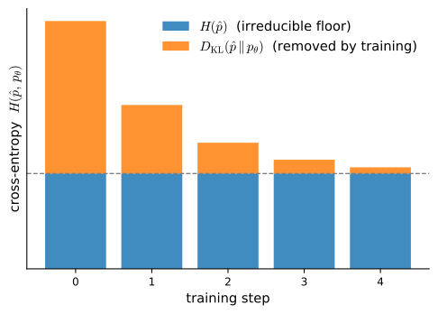
This also explains why minimizing cross-entropy is the right thing to do. Cross-entropy decomposes as \(\textrm{CE}(P,Q)=H(P)+D_{\textrm{KL}}(P\|Q)\), the entropy of \(P\) plus the Kullback–Leibler divergence from \(P\) to \(Q\) (see Section 28.1 for that background). Setting \(P=\hat p_{\textrm{data}}\) and \(Q=p_{\boldsymbol{\theta}}\), the empirical entropy \(H(\hat p_{\textrm{data}})\) is fixed by the data and does not depend on \(\boldsymbol{\theta}\), so minimizing the cross-entropy is identical to minimizing the KL term alone:
\[ \mathop{\mathrm{argmin}}_{\boldsymbol{\theta}}\, \textrm{CE}\!\left(\hat p_{\textrm{data}},\, p_{\boldsymbol{\theta}}\right) = \mathop{\mathrm{argmin}}_{\boldsymbol{\theta}}\, D_{\textrm{KL}}\!\left(\hat p_{\textrm{data}}\,\|\,p_{\boldsymbol{\theta}}\right). \]
For discrete outcomes, maximum likelihood is therefore the KL projection of the empirical distribution onto the model family. This statement is not a literal finite-sample identity for continuous observations: their empirical measure is atomic, and its KL divergence to an absolutely continuous model is infinite. In the continuous case the sample criterion is still the average negative log-density. At the population level it is equivalent to minimizing \(D_{\textrm{KL}}(P_\star\|P_{\boldsymbol{\theta}})\) when the laws have a common dominating measure and the relevant expectations are finite.
That population reading also covers misspecification. If no \(p_{\boldsymbol{\theta}}\) equals the data-generating law, a consistent MLE targets a pseudo-true parameter that minimizes the population KL divergence, provided the minimizer is well defined and the estimator-theory conditions below hold (White 1982). For this fixed discrete empirical distribution, the cross-entropy cannot fall below the constant \(H(\hat p_{\textrm{data}})\); optimization changes only the KL gap, as Figure 27.3.1 shows. This is an algebraic decomposition of the observed frequencies, not by itself a statement about irreducible population randomness. As a special case, the categorical NLL of a classifier with one-hot labels is precisely the softmax cross-entropy loss of Section 3.1.
27.3.2.2 From Probabilities to Densities
The preceding discussion concerned discrete outcomes, where \(P(X\mid\boldsymbol{\theta})\) is a genuine probability. For continuous data we replace probabilities by densities \(p\). The discrete empirical-cross-entropy identity above should not be copied literally: an atomic empirical measure is generally singular with respect to a continuous density, so that KL divergence is infinite. The sample objective remains the average negative log-density, while its population expectation is a cross-entropy and differs from \(D_{\textrm{KL}}(p_\star\|p_{\boldsymbol{\theta}})\) by the fixed differential entropy of the data-generating density when those quantities are finite. The remaining practical issue is that the probability of observing any exact real value is zero, so the naive probability likelihood is \(0\) for every \(\boldsymbol{\theta}\). The resolution is to ask for a match only to within a small tolerance \(\epsilon\), then watch the \(\epsilon\) cancel.
For i.i.d. observations \(x_1,\ldots,x_n\), the probability that each lands in a window of width \(\epsilon\) is, to first order,
\[ P\big(X_i \in [x_i, x_i+\epsilon]\ \forall i \mid \boldsymbol{\theta}\big) \approx \epsilon^n \prod_{i=1}^n p(x_i\mid\boldsymbol{\theta}). \]
Taking the negative log,
\[ -\log P\big(X_i \in [x_i, x_i+\epsilon]\ \forall i\mid\boldsymbol{\theta}\big) \approx -n\log\epsilon - \sum_{i} \log p(x_i\mid\boldsymbol{\theta}). \]
The tolerance enters only through the additive constant \(-n\log\epsilon\), which is free of \(\boldsymbol{\theta}\). Demanding four digits of precision or four hundred changes that constant but never the minimizer, so we drop it and minimize
\[ -\sum_{i} \log p(x_i\mid\boldsymbol{\theta}) \]
exactly as in the discrete case. Thus continuous-data likelihoods use density values in place of probability masses. We next apply this construction to the Gaussian density.
27.3.2.3 Gaussian Negative Log-Likelihood and Mean Squared Error
The most-used regression loss falls out of the same principle by choosing a Gaussian noise model. Suppose each target is the model’s prediction plus Gaussian noise of fixed variance, \(y_i \sim \mathcal{N}(\hat y_i, \sigma^2)\) with \(\hat y_i = f_{\boldsymbol{\theta}}(\mathbf{x}_i)\).
Proposition (Gaussian NLL = MSE). For fixed-variance Gaussian targets, the negative log-likelihood equals the mean squared error up to a constant independent of \(\boldsymbol{\theta}\):
\[ -\log \prod_{i=1}^n \mathcal{N}(y_i;\,\hat y_i,\,\sigma^2) = \frac{1}{2\sigma^2}\sum_{i=1}^n (y_i-\hat y_i)^2 + \frac{n}{2}\log(2\pi\sigma^2). \tag{27.3.4}\]
Hence \(\mathop{\mathrm{argmin}}_{\boldsymbol{\theta}}\) of this NLL is the \(\mathop{\mathrm{argmin}}\) of \(\sum_i (y_i-\hat y_i)^2\).
Proof. The Gaussian density Equation 27.2.10 is \(\mathcal{N}(y;\hat y,\sigma^2) = (2\pi\sigma^2)^{-1/2}\exp\!\big(-(y-\hat y)^2/(2\sigma^2)\big)\). Take its negative log,
\[ -\log \mathcal{N}(y_i;\hat y_i,\sigma^2) = \frac{(y_i-\hat y_i)^2}{2\sigma^2} + \frac{1}{2}\log(2\pi\sigma^2), \]
then sum over the \(n\) independent examples, which is Equation 27.3.4. The second term is the same for every \(\boldsymbol{\theta}\) (the variance is fixed), so it cannot affect the minimizer, and the leading factor \(1/(2\sigma^2)\) is a positive constant. Dropping both leaves \(\sum_i (y_i-\hat y_i)^2\), the sum of squared errors. \(\blacksquare\)
So squared-error regression is maximum likelihood under the assumption that the residuals are Gaussian, the assumption the central limit theorem makes plausible whenever the noise is a sum of many small independent effects (Section 27.2). The same recipe turns every common loss into the NLL of a chosen conditional \(p(y\mid\mathbf x)\): pick the noise model and its negative log is the loss.
| Noise model \(p(y\mid\mathbf x)\) | Negative log-likelihood \(-\log p(y\mid\mathbf x)\) | Deep-learning loss |
|---|---|---|
| Gaussian, fixed variance | \(\tfrac{1}{2\sigma^2}(y-\hat y)^2 + \textrm{const}\) | mean squared error (MSE) |
| Bernoulli | \(-\,y\log\hat p - (1-y)\log(1-\hat p)\) | binary cross-entropy (BCE) |
| Categorical (one-hot \(y\)) | \(-\sum_k y_k \log \hat p_k\) | softmax cross-entropy |
| Laplace, fixed scale | \(\tfrac{1}{b}\lvert y-\hat y\rvert + \textrm{const}\) | mean absolute error (MAE) |
Each row follows by taking the negative logarithm of the density and omitting terms independent of \(\boldsymbol{\theta}\). Thus the choice of loss encodes an assumption about the conditional distribution of the observations.
27.3.3 Estimator Theory: Why Maximum Likelihood Works
How good is \(\hat{\boldsymbol{\theta}}\)? Suppose the observations are i.i.d. and the data-generating distribution belongs to the model. The average NLL then estimates the expected negative log-likelihood. When the laws have a common dominating measure and the expectations are finite, this population objective differs from a KL divergence by a constant and is minimized at the truth \(\boldsymbol{\theta}=\boldsymbol{\theta}^\star\), where the KL term vanishes. This conclusion requires the model to be identifiable, meaning distinct parameters give distinct distributions, \(\boldsymbol{\theta}\neq\boldsymbol{\theta}'\Rightarrow p_{\boldsymbol{\theta}}\neq p_{\boldsymbol{\theta}'}\); otherwise several parameters tie for the minimum and “the” true parameter is not even well defined. Neural networks are generally not identifiable: permuting the hidden units of a layer (together with their weights) changes the parameter vector but not the function it computes, so for such models consistency can only ever be a statement about the fitted distribution \(p_{\hat{\boldsymbol{\theta}}}\), never about the parameter vector itself.
Minimizing the empirical average therefore targets the right minimizer. One caveat: the law of large numbers makes the empirical objective converge to the population one at each fixed \(\boldsymbol{\theta}\), and pointwise convergence of objectives does not by itself force their minimizers to converge. For that, the convergence must be uniform over the parameter space: the supremum over \(\boldsymbol{\theta}\) of the gap between the empirical and population objectives must go to zero. With a unique population optimum and uniform convergence in hand (often obtained from continuity plus compactness or a suitable coercivity condition), the conclusion is a theorem (Wasserman 2013): for a well-specified, identifiable model the MLE is consistent, converging in probability to the true parameter, \(\hat{\boldsymbol{\theta}}\xrightarrow{P}\boldsymbol{\theta}^\star\), so the probability of an error larger than any fixed tolerance goes to zero. The coin made this concrete: \(\hat\theta = n_H/(n_H+n_T) \to \theta^\star\) directly by the law of large numbers, and the Bernoulli family is identifiable, since different biases give different distributions. Consistency, asymptotic unbiasedness, and efficiency are the estimator-quality notions that Section 27.5 develops systematically; here they appear specialized to the MLE.
Consistency says only where \(\hat{\boldsymbol{\theta}}\) lands; the sharper statement is how fast and how tightly it concentrates. Under the regularity conditions stated below, the MLE is asymptotically normal: the rescaled error converges in distribution to a Gaussian,
\[ \sqrt{n}\,\big(\hat{\boldsymbol{\theta}} - \boldsymbol{\theta}^\star\big) \;\xrightarrow{d}\; \mathcal{N}\!\big(\mathbf{0},\; I(\boldsymbol{\theta}^\star)^{-1}\big), \tag{27.3.5}\]
where \(I(\boldsymbol{\theta})\) is the Fisher information defined just below (Bishop 2006; Wasserman 2013). Here and below, “regularity conditions” means one standard package of hypotheses that we state once and take on faith: the density is sufficiently differentiable in \(\boldsymbol{\theta}\) that differentiation and integration can be interchanged (the tool of Section 25.4), the support of \(p(x\mid\boldsymbol{\theta})\) does not depend on \(\boldsymbol{\theta}\), and the true parameter lies in the interior of the parameter space. The Fisher information must also be finite and nonsingular, and the score must satisfy the needed moment conditions (Wasserman 2013). The display says two things. First, the error shrinks at the \(1/\sqrt{n}\) rate, so the standard error of each component falls like \(1/\sqrt n\): halving it costs four times the data. Second, the limiting variance is exactly \(I(\boldsymbol{\theta}^\star)^{-1}\), and the Cramér–Rao bound stated below (Equation 27.3.7) says no unbiased estimator can have smaller variance than \(I(\boldsymbol{\theta}^\star)^{-1}/n\). The MLE attains the Cramér–Rao floor in the limit: it is asymptotically efficient, asymptotically the best unbiased estimator. The qualifiers matter. At finite \(n\) the MLE is generally only asymptotically unbiased, not exactly unbiased: the maximum-likelihood estimate of a Gaussian’s variance divides the sum of squares by \(n\) rather than \(n-1\) and so systematically underestimates \(\sigma^2\). Section 27.5 works out exactly this bias, identifying the \(n\)-divided estimator as the Gaussian MLE, when it derives the \(n-1\) correction. Maximum likelihood is optimal in the limit within this regular setting, not a guarantee of unbiasedness at every sample size. Parameters on a boundary, singular information, mixtures, and many overparameterized neural networks can have different limiting behavior.
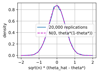
Watching the theorem happen. Asymptotic normality is the section’s central limit theorem, and like the CLT proper it can be watched. The cell below returns to the coin: it draws \(20{,}000\) independent datasets of \(n=400\) flips with true bias \(\theta^\star=0.7\), computes the MLE \(\hat\theta=n_H/n\) on each, and histograms the rescaled errors \(\sqrt n\,(\hat\theta-\theta^\star)\) against the Gaussian that Equation 27.3.5 names. One scope note: the coin’s MLE is itself a sample mean, so for the coin the theorem reduces to the CLT proper; the demonstration illustrates the general statement on the one model where we can also verify it by hand. For the coin the Fisher information works out below to \(I(\theta)=1/(\theta(1-\theta))\), so the predicted limit is \(\mathcal N\bigl(0,\ \theta^\star(1-\theta^\star)\bigr)\) with variance \(0.21\), and the histogram lands on that particular Gaussian, center, width, and height. (One numerical nicety: \(\hat\theta\) lives on the lattice \(k/n\), so we offset the bin edges by half a lattice step to keep the discrete values off the edges.)
rng = onp.random.default_rng(0)
theta_star, n, reps = 0.7, 400, 20000
flips = rng.random((reps, n)) < theta_star             # 20,000 datasets at once
z = onp.sqrt(n) * (flips.mean(axis=1) - theta_star)    # sqrt(n)(theta_hat - theta*)
sigma2 = theta_star * (1 - theta_star)                 # = 1 / I(theta*)
hist, edges = onp.histogram(z, bins=40, range=(-2.025, 1.975), density=True)
x = onp.arange(-2, 2, 0.01)
d2l.plot(x, [onp.interp(x, (edges[:-1] + edges[1:]) / 2, hist),
             onp.exp(-x**2 / (2 * sigma2)) / onp.sqrt(2 * onp.pi * sigma2)],
         xlabel='sqrt(n) * (theta_hat - theta*)', ylabel='density',
         legend=['20,000 replications', 'N(0, theta*(1-theta*))'])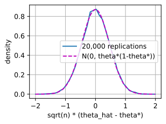
27.3.3.1 Fisher Information and the Score
To make Equation 27.3.5 quantitative we need the object \(I(\boldsymbol{\theta})\) it contains. Define the score as the gradient of the log-likelihood with respect to the parameters, \(s(x;\boldsymbol{\theta}) = \nabla_{\boldsymbol{\theta}} \log p(x\mid\boldsymbol{\theta})\). The score is the per-example version of the NLL gradient we already met: setting \(\sum_i s(x_i;\boldsymbol{\theta}) = \mathbf 0\) is exactly the first-order condition that locates \(\hat{\boldsymbol{\theta}}\). At the true parameter the score has mean zero: differentiating the normalization \(\int p(x\mid\boldsymbol{\theta})\,dx = 1\) under the integral sign gives
\[ \mathbf 0 = \nabla_{\boldsymbol{\theta}} \int p(x\mid\boldsymbol{\theta})\,dx = \int \nabla_{\boldsymbol{\theta}}\, p(x\mid\boldsymbol{\theta})\,dx = \int s(x;\boldsymbol{\theta})\, p(x\mid\boldsymbol{\theta})\,dx = \mathbb{E}_{\boldsymbol{\theta}}\!\big[\,s(x;\boldsymbol{\theta})\,\big], \]
exactly the computation of Section 25.4, which also grants the interchange of derivative and integral (the first of the regularity conditions named above); the third equality is the identity \(\nabla_{\boldsymbol{\theta}}\, p = p\,\nabla_{\boldsymbol{\theta}} \log p = p\,s\). Because the score has mean zero, its variance equals its second moment, and that variance is the Fisher information (Fisher 1925),
\[ I(\boldsymbol{\theta}) = \operatorname{Var}_{\boldsymbol{\theta}}\!\big[\,s(x;\boldsymbol{\theta})\,\big] = \mathbb{E}_{\boldsymbol{\theta}}\!\big[\,s(x;\boldsymbol{\theta})\,s(x;\boldsymbol{\theta})^\top\,\big] = -\,\mathbb{E}_{\boldsymbol{\theta}}\!\big[\nabla^2_{\boldsymbol{\theta}} \log p(x\mid\boldsymbol{\theta})\big]. \tag{27.3.6}\]
The middle equality is the mean-zero property at work: \(\operatorname{Var}[s]=\mathbb E[ss^\top]\) once \(\mathbb E[s]=\mathbf 0\). The last equality is the information identity, and it follows by differentiating \(\mathbb{E}_{\boldsymbol{\theta}}[s]=\mathbf 0\) once more, with the same interchange granted. The product rule splits the derivative into two terms,
\[ \mathbf 0 = \nabla_{\boldsymbol{\theta}} \int s(x;\boldsymbol{\theta})\,p(x\mid\boldsymbol{\theta})\,dx = \int \nabla^2_{\boldsymbol{\theta}} \log p(x\mid\boldsymbol{\theta})\; p(x\mid\boldsymbol{\theta})\,dx + \int s(x;\boldsymbol{\theta})\,\big(\nabla_{\boldsymbol{\theta}}\, p(x\mid\boldsymbol{\theta})\big)^\top dx, \]
and substituting \(\nabla_{\boldsymbol{\theta}}\, p = p\,s\) in the second term turns it into \(\mathbb{E}_{\boldsymbol{\theta}}[\,s\,s^\top]\), so
\[ \mathbb{E}_{\boldsymbol{\theta}}\!\big[\nabla^2_{\boldsymbol{\theta}} \log p(x\mid\boldsymbol{\theta})\big] + \mathbb{E}_{\boldsymbol{\theta}}\!\big[\,s\,s^\top\,\big] = \mathbf 0, \]
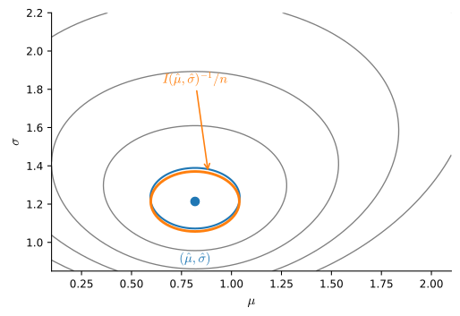
which is the last equality of Equation 27.3.6 rearranged. The identity says that the information is the expected curvature of the NLL. The reading is intuitive: a sharply peaked log-likelihood (large curvature, large \(I\)) pins the parameter down tightly, so the estimate has small variance; a flat one leaves \(\boldsymbol{\theta}\) poorly determined. That is precisely what Equation 27.3.5 says, \(\operatorname{Var}(\hat{\boldsymbol{\theta}}) \approx I(\boldsymbol{\theta}^\star)^{-1}/n\). Figure 27.3.2 draws the picture for a Gaussian’s two parameters: the NLL is a bowl around the MLE, and the inverse of its curvature is the ellipse within which the estimate scatters.
The curvature intuition extends to a theorem constraining every estimator. The Cramér–Rao bound (Cramér 1946; Radhakrishna Rao 1945) states that any unbiased estimator \(\tilde\theta\) built from \(n\) i.i.d. observations obeys
\[ \operatorname{Var}\big(\tilde\theta\big) \;\ge\; \frac{1}{n\,I(\theta)} \tag{27.3.7}\]
(stated here for a scalar parameter; for vectors the statement reads \(\operatorname{Cov}(\tilde{\boldsymbol{\theta}}) \succeq I(\boldsymbol{\theta})^{-1}/n\) in the positive-semidefinite order) (Wasserman 2013). Information caps precision: no cleverness in constructing the estimator can beat the curvature the model itself supplies, and comparing with Equation 27.3.5 shows the MLE’s limiting variance meets the Cramér–Rao floor exactly, which is precisely the asymptotic efficiency claimed above.
Back to the coin. A single flip has log-likelihood \(\log p(x\mid\theta) = x\log\theta + (1-x)\log(1-\theta)\) for \(x\in\{0,1\}\), so the score and its derivative are
\[ s(x;\theta) = \frac{x}{\theta} - \frac{1-x}{1-\theta}, \qquad \frac{d}{d\theta}\, s(x;\theta) = -\frac{x}{\theta^2} - \frac{1-x}{(1-\theta)^2}. \]
Taking \(-\mathbb{E}[\,\cdot\,]\) with \(\mathbb{E}[x]=\theta\) collapses the two fractions to \(\tfrac{1}{\theta} + \tfrac{1}{1-\theta}\), so the per-flip Fisher information and its inverse are
\[ I(\theta) = \frac{1}{\theta} + \frac{1}{1-\theta} = \frac{1}{\theta(1-\theta)}, \qquad \frac{I(\theta)^{-1}}{n} = \frac{\theta(1-\theta)}{n}. \tag{27.3.8}\]
Note that the per-flip information \(1/(\theta(1-\theta))\) is smallest at \(\theta = 1/2\): fair coins are the hardest to pin down, each flip carrying the least information about the bias. The prediction of Equation 27.3.5 is that the MLE \(\hat\theta = n_H/n\) over \(n\) flips has variance about \(\theta(1-\theta)/n\), which, by Equation 27.3.8, is also the Cramér–Rao floor Equation 27.3.7 for this problem. We can check that this is exactly right here (\(\hat\theta\) is a scaled binomial count, whose variance is \(\theta(1-\theta)/n\) on the nose) and confirm it by simulation: run the \(n\)-flip experiment many times and compare the spread of the resulting estimates to the floor.
# NumPy simulation of the coin MLE's variance.
theta_star, n, trials = 0.3, 200, 20000
rng = onp.random.default_rng(0)
# Each trial: flip the coin n times; the MLE is the observed head fraction.
heads = rng.binomial(n, theta_star, size=trials)
theta_hats = heads / n

empirical_var = theta_hats.var()
cramer_rao = theta_star * (1 - theta_star) / n  # = I(theta)^-1 / n
empirical_var, cramer_rao(np.float64(0.0010385371777499998), 0.00105)(np.float64(0.0010385371777499998), 0.00105)(np.float64(0.0010385371777499998), 0.00105)(0.00103853717775, 0.00105)The empirical variance of the maximum-likelihood estimates matches the Cramér–Rao floor \(\theta(1-\theta)/n\) to two digits: the coin’s MLE is as tight as Equation 27.3.7 permits. This is asymptotic efficiency made concrete, and it is why the curvature of a loss surface (its Fisher information, or empirically its Hessian) quantifies the local uncertainty of a fitted parameter.
27.3.4 MAP Estimation and Regularization
Maximum likelihood does not use a prior over parameters. Introducing a prior \(P(\boldsymbol{\theta})\) leads instead to maximum a posteriori (MAP) estimation. Its negative logarithm appears in the optimization objective as a regularizer. Maximizing the full posterior Equation 27.3.9 and taking negative logs,
\[ \hat{\boldsymbol{\theta}}_{\textrm{MAP}} = \mathop{\mathrm{argmax}}_{\boldsymbol{\theta}}\, P(X\mid\boldsymbol{\theta})\,P(\boldsymbol{\theta}) = \mathop{\mathrm{argmin}}_{\boldsymbol{\theta}}\, \Big[\underbrace{-\textstyle\sum_i \log p(x_i\mid\boldsymbol{\theta})}_{\textrm{data fit (NLL)}} \;\underbrace{-\log P(\boldsymbol{\theta})}_{\textrm{regularizer}}\Big]. \tag{27.3.9}\]
The objective is the familiar data-fit term plus a penalty: the negative log-prior. A prior concentrated near small parameters penalizes large ones, which is precisely what a regularizer does.
27.3.4.1 Gaussian Priors and Weight Decay
Proposition (Gaussian prior = \(L_2\) / weight decay). A Gaussian prior \(\boldsymbol{\theta}\sim\mathcal{N}(\mathbf 0,\tau^2 \mathbf I)\) contributes the penalty \(\tfrac{1}{2\tau^2}\lVert\boldsymbol{\theta}\rVert_2^2\) to the MAP objective. With Gaussian-noise data (variance \(\sigma^2\)), MAP estimation is \(L_2\)-regularized least squares with weight-decay strength \(\lambda = \sigma^2/\tau^2\).
Proof. The density of \(\mathcal{N}(\mathbf 0,\tau^2\mathbf I)\) is proportional to \(\exp\!\big(-\lVert\boldsymbol{\theta}\rVert_2^2/(2\tau^2)\big)\), so its negative log-prior is \(\tfrac{1}{2\tau^2}\lVert\boldsymbol{\theta}\rVert_2^2\) plus a constant. Insert this and the Gaussian NLL Equation 27.3.4 into the MAP objective Equation 27.3.9:
\[ \hat{\boldsymbol{\theta}}_{\textrm{MAP}} = \mathop{\mathrm{argmin}}_{\boldsymbol{\theta}}\; \frac{1}{2\sigma^2}\sum_{i}(y_i-\hat y_i)^2 + \frac{1}{2\tau^2}\lVert\boldsymbol{\theta}\rVert_2^2 . \]
Multiplying by the positive constant \(2\sigma^2\) leaves \(\sum_i(y_i-\hat y_i)^2 + \tfrac{\sigma^2}{\tau^2}\lVert\boldsymbol{\theta}\rVert_2^2\), which is ridge regression (Section 2.7) with \(\lambda=\sigma^2/\tau^2\). \(\blacksquare\)
This is the probabilistic origin of weight decay: the regularizer we add by hand in Section 2.7, and read as a norm constraint in Section 26.4.4.5, is the negative log of a Gaussian belief that weights should be small. The same construction with a Laplace prior \(p(\boldsymbol{\theta})\propto e^{-\lVert\boldsymbol{\theta}\rVert_1/b}\) gives the \(L_1\) penalty \(\tfrac{1}{b}\lVert\boldsymbol{\theta}\rVert_1\), whose kink at the origin produces exact zeros, i.e. sparsity. Figure 27.3.3 shows the resulting compromise: the NLL favors the MLE, the negative log-prior favors the prior mean, and the MAP estimate lies between them.
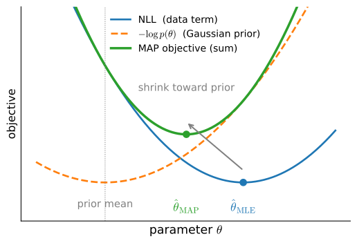
The figure also reads off the two limits. As the prior flattens (\(\tau\to\infty\), or \(b\to\infty\)) the penalty vanishes and \(\hat{\boldsymbol{\theta}}_{\textrm{MAP}} \to \hat{\boldsymbol{\theta}}_{\textrm{MLE}}\), the flat-prior assumption we started with. And as the data grows the NLL term deepens faster than the fixed prior, so the data term dominates and MAP again approaches the MLE. A bookkeeping detail makes the second limit quantitative: deep-learning code minimizes the mean per-example loss rather than the sum, and dividing the MAP objective by \(n\) rescales the weight decay to \(\lambda = \sigma^2/(n\tau^2)\): the prior’s contribution to the averaged loss decreases as \(1/n\). Regularization matters most precisely when data is scarce.
27.3.4.2 A Beta Prior on the Coin
We now return to the coin example. A prior on its bias must have support on \([0,1]\); a common choice is the Beta distribution \(p(\theta)\propto\theta^{a-1}(1-\theta)^{b-1}\) with shape parameters \(a, b > 0\), the conjugate prior of Section 27.2: multiplying by the likelihood Equation 27.3.2 shifts the exponents by the observed counts, so the posterior is again a Beta (Equation 27.2.18),
\[ P(\theta\mid X) \;\propto\; \theta^{\,n_H + a - 1}\,(1-\theta)^{\,n_T + b - 1}. \]
MAP asks for the mode of this density. That is the same single-variable maximization we solved for the likelihood itself: the posterior has the shape \(\theta^{\alpha}(1-\theta)^{\beta}\) with \(\alpha = n_H+a-1\) and \(\beta = n_T+b-1\), and whenever both exponents are positive (e.g. \(a, b \ge 1\) on our data) the maximum is interior. The answer is therefore the same ratio, “head exponent over total exponent”:
\[ \hat\theta_{\textrm{MAP}} \;=\; \frac{n_H + a - 1}{n + a + b - 2}, \qquad n = n_H + n_T. \tag{27.3.10}\]
The reading is pseudo-counts: the prior behaves exactly like \(a-1\) phantom heads and \(b-1\) phantom tails appended to the data before taking the empirical frequency. A \(\mathrm{Beta}(2,2)\) prior adds one phantom flip of each kind, turning our \(9\)-of-\(13\) coin into \((9+1)/(13+2) = 2/3\), pulled from \(9/13\approx 0.692\) toward \(1/2\); a \(\mathrm{Beta}(30,30)\) prior would all but pin the estimate near a fair coin until the data outweighed its \(58\) phantom flips. And as \(n\) grows, any fixed stock of phantom flips washes out: \(\hat\theta_{\textrm{MAP}}\to\hat\theta_{\textrm{MLE}}\), the data-swamps-the-prior limit we just met.
Two subtleties in Equation 27.3.10 are easy to get wrong. First, the flat prior \(\mathrm{Beta}(1,1)\), uniform on \([0,1]\), gives \(\hat\theta_{\textrm{MAP}} = n_H/n\): MAP under a uniform prior is exactly the MLE, zero phantom flips, no smoothing at all. In particular the “add-one” (Laplace) smoothing rule \((n_H+1)/(n+2)\) is not the uniform-prior MAP; read as pseudo-counts, it is the MAP under \(\mathrm{Beta}(2,2)\).
Second, the mode is not the mean. The posterior mean is
\[ \mathbb{E}[\theta\mid X] \;=\; \frac{n_H + a}{n + a + b}, \]
which under the flat prior becomes \((n_H+1)/(n+2)\): Laplace’s rule of succession (Laplace 1814), precisely the add-one rule. So add-one smoothing is a Bayes estimate under the uniform prior, but it uses a different summary: the posterior mean, not the posterior mode. (Numerically it coincides with the \(\mathrm{Beta}(2,2)\) mode, which is why the two are so often conflated.) Naive Bayes (Section 27.7) uses this smoothing to keep never-observed feature–class pairs from annihilating its products; the pseudo-count interpretation explains the correction.
27.3.4.3 Distinguishing the Posterior Mode from the Posterior
One caution before we move on: MAP is not the same as “being Bayesian.” MAP restores the prior but still reports a single point: the mode of the posterior \(P(\boldsymbol{\theta}\mid X)\), the same \(\mathop{\mathrm{argmax}}\) as in Equation 27.3.9. Genuine Bayesian inference keeps the entire posterior distribution and integrates over it, predicting with the posterior-averaged \(\int p(x\mid\boldsymbol{\theta})\,P(\boldsymbol{\theta}\mid X)\,d\boldsymbol{\theta}\) rather than plugging in one \(\hat{\boldsymbol{\theta}}_{\textrm{MAP}}\). That average propagates parameter uncertainty into the prediction, where the mode discards it. The mode is not even reparameterization-invariant, since a nonlinear change of variables moves the peak of a density but not its integral. Maximum likelihood is instead equivariant under reparameterization, meaning that if \(\hat\theta\) is the MLE of \(\theta\), then \(g(\hat\theta)\) is the MLE of \(g(\theta)\) for any one-to-one \(g\). For example, the MLE of the coin’s log-odds is \(\log\frac{9/13}{4/13} = \log\frac{9}{4}\) (Wasserman 2013). The reason is that relabeling the parameter axis moves no maximum: likelihood values are attached to points, while densities carry a Jacobian. MAP inherits the prior density’s Jacobian, and with it the dependence on how the parameter happens to be written down. Marginalizing over the posterior is its own subject, beyond our scope here (Murphy 2022; MacKay 2003); the point is only that MAP is one more point estimate (maximum likelihood with a penalty) and should not be mistaken for the full Bayesian treatment.
27.3.5 Latent Variables, EM, and the ELBO
The preceding section concerned the statistical behavior of an optimizer of the likelihood. We now turn to a computational obstacle: in latent-variable models, evaluating or optimizing that likelihood can itself be difficult.
Every likelihood so far has been a product of terms we could log and differentiate directly. The most interesting generative models are not so obliging. They posit a latent variable \(z\) (an unobserved cluster identity, a topic, the “seed” a generator decodes into an image) and define the joint distribution
\[ p(x, z; \boldsymbol{\theta}) = p(z; \boldsymbol{\theta})\, p(x \mid z; \boldsymbol{\theta}), \]
of which we observe only \(x\). The likelihood of an observation is then a marginal, obtained by summing (for continuous latents, integrating) the latent out:
\[ p(x;\boldsymbol{\theta}) = \sum_{z} p(z;\boldsymbol{\theta})\, p(x\mid z;\boldsymbol{\theta}). \tag{27.3.11}\]
27.3.5.1 The Difficulty Introduced by Latent Variables
The canonical example is the Gaussian mixture model (GMM): the latent \(z \in \{1,\ldots,K\}\) picks a component with probability \(P(z = k) = \pi_k\), and the observation is then drawn from that component, \(x \mid z{=}k \sim \mathcal{N}(\mu_k, \sigma_k^2)\). The data’s NLL is
\[ \ell(\boldsymbol{\theta}) = -\sum_{i=1}^n \log\Big(\sum_{k=1}^K \pi_k\, \mathcal{N}(x_i;\, \mu_k, \sigma_k^2)\Big), \qquad \boldsymbol{\theta} = (\pi_k, \mu_k, \sigma_k)_{k=1}^K. \]
The trouble is the sum inside the logarithm. Until now every log reached an individual density and the NLL split into per-example, per-parameter pieces; here the log stops at the mixture, every parameter appears inside every term through the shared sum, and no closed form solves the first-order conditions. Contrast the complete-data problem: if an oracle revealed each \(z_i\), the likelihood would factor by component, and maximum likelihood would collapse to the estimators we already own: the fraction of points in component \(k\) for \(\pi_k\) (the coin), and the per-component sample mean and variance for \(\mu_k, \sigma_k^2\) (the Gaussian). Plain gradient descent on \(\ell(\boldsymbol{\theta})\) remains possible, but the structure of the problem (easy if complete, hard only because \(z\) is missing) suggests something better: guess the missing labels probabilistically, then solve the easy problem.
27.3.5.2 The Evidence Lower Bound
Let \(q(z)\) be any distribution over the latent with \(q(z) > 0\) wherever \(p(x,z;\boldsymbol{\theta}) > 0\), our probabilistic guess. Insert it into the marginal and apply Jensen’s inequality (\(\log\) is concave, so \(\log \mathbb{E}[\cdot] \ge \mathbb{E}[\log(\cdot)]\); Section 26.3.3):
\[ \log p(x;\boldsymbol{\theta}) = \log \sum_z q(z)\, \frac{p(x,z;\boldsymbol{\theta})}{q(z)} \;\ge\; \sum_z q(z) \log \frac{p(x,z;\boldsymbol{\theta})}{q(z)} \;=:\; \mathcal{L}(q, \boldsymbol{\theta}). \tag{27.3.12}\]
The right-hand side is the evidence lower bound ELBO. The name comes from calling the marginal log-likelihood \(\log p(x;\boldsymbol{\theta})\) the evidence: for the latent \(z\) it plays exactly the role the denominator \(P(X)\) played for the parameters in Bayes’ rule at the start of this section, namely the marginal probability of what we actually observed. Expanding the fraction splits the bound into two readable pieces,
\[ \mathcal{L}(q,\boldsymbol{\theta}) = \mathbb{E}_{q}\big[\log p(x,z;\boldsymbol{\theta})\big] + H(q), \]
the expected complete-data log-likelihood (the easy objective, averaged over the guess) plus the entropy of the guess, which does not involve \(\boldsymbol{\theta}\) at all (Section 28.1). How much does the bound give away? Exactly a KL divergence:
Proposition (the ELBO gap is a KL). For every \(q\) and every \(\boldsymbol{\theta}\),
\[ \log p(x;\boldsymbol{\theta}) = \mathcal{L}(q,\boldsymbol{\theta}) + D_{\textrm{KL}}\big(q(z)\,\|\,p(z\mid x;\boldsymbol{\theta})\big). \tag{27.3.13}\]
Hence \(\mathcal{L}(q,\boldsymbol{\theta}) \le \log p(x;\boldsymbol{\theta})\), with equality if and only if \(q\) is the posterior \(p(z\mid x;\boldsymbol{\theta})\).
Proof. Expand the KL term using Bayes’ rule, \(p(z\mid x;\boldsymbol{\theta}) = p(x,z;\boldsymbol{\theta})/p(x;\boldsymbol{\theta})\):
\[ D_{\textrm{KL}}\big(q \,\|\, p(z\mid x;\boldsymbol{\theta})\big) = \mathbb{E}_q\!\left[\log \frac{q(z)\, p(x;\boldsymbol{\theta})}{p(x,z;\boldsymbol{\theta})}\right] = \log p(x;\boldsymbol{\theta}) - \mathcal{L}(q,\boldsymbol{\theta}), \]
where \(\log p(x;\boldsymbol{\theta})\) exits the expectation because it does not involve \(z\). Rearranging gives Equation 27.3.13; since the KL divergence is nonnegative and vanishes exactly when its arguments agree, the bound and its equality condition follow. \(\blacksquare\)
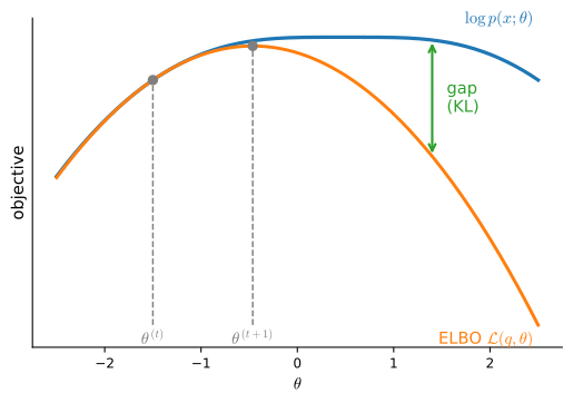
Figure 27.3.4 draws the resulting geometry: for a fixed guess the ELBO is a curve running everywhere below the evidence, and choosing \(q\) well pinches the two together at the current parameters.
27.3.5.3 Expectation–Maximization
The proposition turns the intractable problem into coordinate ascent on \(\mathcal{L}(q, \boldsymbol{\theta})\): maximize over one of the two arguments while the other is held fixed, then swap, and repeat. For a dataset \(X = \{x_1,\ldots,x_n\}\) of independent observations the bound applies example by example and sums, with one guess \(q_i\) per data point. The expectation–maximization (EM) algorithm alternates the two coordinates (Dempster et al. 1977):
E-step. Hold \(\boldsymbol{\theta}^{(t)}\) fixed and maximize over the guesses: by the equality condition of Equation 27.3.13, the best \(q_i\) is the posterior, \(q_i^{(t)}(z) = p(z \mid x_i; \boldsymbol{\theta}^{(t)})\). This closes every gap, making the bound tight: \(\sum_i \mathcal{L}(q_i^{(t)}, \boldsymbol{\theta}^{(t)}) = \log p(X;\boldsymbol{\theta}^{(t)})\).
M-step. Hold the guesses fixed and maximize over the parameters:
\[ \boldsymbol{\theta}^{(t+1)} = \mathop{\mathrm{argmax}}_{\boldsymbol{\theta}} \sum_i \mathbb{E}_{q_i^{(t)}}\big[\log p(x_i, z; \boldsymbol{\theta})\big] \]
(the entropy terms do not involve \(\boldsymbol{\theta}\)). This is the easy, complete-data objective, with soft assignments standing in for the oracle’s labels.
Proposition (EM never decreases the likelihood). Each EM iteration satisfies \(\log p(X;\boldsymbol{\theta}^{(t+1)}) \ge \log p(X;\boldsymbol{\theta}^{(t)})\).
Proof. Chain three facts:
\[ \log p(X;\boldsymbol{\theta}^{(t+1)}) \;\ge\; \sum_i \mathcal{L}\big(q_i^{(t)}, \boldsymbol{\theta}^{(t+1)}\big) \;\ge\; \sum_i \mathcal{L}\big(q_i^{(t)}, \boldsymbol{\theta}^{(t)}\big) \;=\; \log p(X;\boldsymbol{\theta}^{(t)}). \]
The first inequality is the ELBO bound Equation 27.3.12 at the new parameters; the second is the definition of the M-step; the equality is the tightness the E-step bought. \(\blacksquare\)
For the Gaussian mixture both steps are closed-form. The E-step computes responsibilities, the posterior probability that point \(i\) came from component \(k\),
\[ r_{ik} = \frac{\pi_k\, \mathcal{N}(x_i;\, \mu_k, \sigma_k^2)} {\sum_{j} \pi_j\, \mathcal{N}(x_i;\, \mu_j, \sigma_j^2)}, \]
and the M-step refits each component by responsibility-weighted counting and averaging: with effective counts \(n_k = \sum_i r_{ik}\),
\[ \pi_k = \frac{n_k}{n}, \qquad \mu_k = \frac{1}{n_k}\sum_{i} r_{ik}\, x_i, \qquad \sigma_k^2 = \frac{1}{n_k}\sum_{i} r_{ik}\,(x_i - \mu_k)^2. \tag{27.3.14}\]
These are the coin’s counting estimator and the Gaussian’s mean and variance estimators, softened: instead of voting for one component, each point spreads its single vote across components in proportion to its responsibilities (exercise 10 derives the \(\mu_k\) update). The cell below runs EM on a two-component mixture in plain NumPy and prints the log-likelihood as it climbs.
# EM for a two-component 1-D Gaussian mixture, in plain numpy.
rng = onp.random.default_rng(42)
# 300 points from N(-2, 0.8^2) and 200 from N(1.5, 0.6^2)
x = onp.concatenate([rng.normal(-2.0, 0.8, 300), rng.normal(1.5, 0.6, 200)])

def gauss(x, mu, sigma):
    return onp.exp(-0.5 * ((x - mu) / sigma)**2) / (sigma * onp.sqrt(2 * onp.pi))

# Deliberately poor start: equal weights, overlapping components
pi, mu, sigma = onp.array([0.5, 0.5]), onp.array([-0.5, 0.5]), onp.array([1.0, 1.0])
for step in range(31):
    # E-step: responsibilities r[i, k], the posterior of component k given x_i
    joint = pi * gauss(x[:, None], mu, sigma)
    r = joint / joint.sum(axis=1, keepdims=True)
    if step % 5 == 0:  # the log-likelihood never decreases
        print(f'step {step:2d}, log-likelihood {onp.log(joint.sum(axis=1)).sum():.2f}')
    # M-step: refit each component by responsibility-weighted averaging
    n_k = r.sum(axis=0)
    pi, mu = n_k / len(x), (r * x[:, None]).sum(axis=0) / n_k
    sigma = onp.sqrt((r * (x[:, None] - mu)**2).sum(axis=0) / n_k)
print(f'pi = {pi.round(3)}, mu = {mu.round(3)}, sigma = {sigma.round(3)}')
step 0, log-likelihood -1289.53
step 5, log-likelihood -845.69
step 10, log-likelihood -845.45
step 15, log-likelihood -845.45
step 20, log-likelihood -845.45
step 25, log-likelihood -845.45
step 30, log-likelihood -845.45
pi = [0.594 0.406], mu = [-2.055 1.494], sigma = [0.715 0.625]The trace behaves exactly as the proposition demands: the log-likelihood rises monotonically, gains most of its ground in the first few iterations, and then flatlines at a stationary point; the recovered weights, means, and scales land near the generating values \((0.6, 0.4)\), \((-2, 1.5)\), \((0.8, 0.6)\), the small residual gaps being finite-sample error, not a failure of EM. Two cautions temper the success. EM is ascent, not global optimization: the mixture likelihood is multimodal (at minimum because relabeling the components permutes the parameters without changing the model, the same identifiability failure we met in the estimator theory above), and EM can stall at a poor local maximum, so practice restarts it from several initializations. And strictly speaking the GMM likelihood is unbounded: let one component collapse onto a single data point with \(\sigma_k \to 0\). Monotonicity itself guarantees only nondecrease; because this objective is unbounded, the values may diverge rather than approach a finite limit. With a variance floor or prior making the relevant level set bounded, plus standard continuity and regularity conditions, EM limit points are stationary (Wu 1983).
The monotonicity proof assumes an exact E-step and an M-step that maximizes (or at least increases) the displayed bound. Approximate inference and stochastic updates, as used in larger models, do not automatically inherit monotonic observed-data likelihood; their guarantees must be established for the particular approximation and update rule.
The bound, not the closed-form M-step, is the part that scales. A variational autoencoder (Kingma and Welling 2014) keeps the ELBO but replaces the per-point E-step with a neural network \(q_{\boldsymbol{\phi}}(z\mid x)\), an amortized guess trained jointly with the generator by stochastic gradient ascent on the ELBO, because for a deep decoder the true posterior is no longer available in closed form. Diffusion models walk further down the same road: their training objective is the ELBO of a deep chain of latent variables (Section 29.4). And the two divergences in this section are deliberately mirrored: Section 28.2 recasts maximum likelihood itself as forward-KL minimization, while the ELBO gap Equation 27.3.13 measures the guess against the posterior in the reverse orientation, \(D_{\textrm{KL}}(q\,\|\,p)\). The distinction has real modelling consequences, taken up in detail there.
27.3.6 Summary
- The maximum likelihood principle directly picks the parameter that maximizes the observed-data probability or density, \(\mathop{\mathrm{argmax}}_{\boldsymbol{\theta}}P(X\mid\boldsymbol{\theta})\). It does not require a prior; MAP is a separate posterior-mode rule that coincides with MLE under a constant prior in the chosen parameterization.
- We optimize the negative log-likelihood \(-\sum_i \log p(x_i\mid\boldsymbol{\theta})\): the log fixes underflow and makes gradients an additive sum, while the sign flip turns “maximize probability” into “minimize a loss.”
- For discrete outcomes, the average NLL is the cross-entropy from the empirical frequencies to the model and differs from the corresponding KL by a fixed empirical entropy. For continuous data, use the average negative log-density at the sample; the clean KL-projection statement is a population statement under suitable integrability conditions. Categorical NLL is softmax cross-entropy, fixed-variance Gaussian NLL is mean squared error, and a Laplace model gives mean absolute error: picking a loss is picking a noise model.
- In a well-specified identifiable model, with a unique population optimum and uniform convergence, the MLE is consistent. Under the additional smoothness, interior-point, moment, and nonsingular-information conditions stated in the text, it is asymptotically normal with limiting variance the inverse Fisher information \(I(\boldsymbol{\theta}^\star)^{-1}/n\), so it attains the Cramér–Rao bound Equation 27.3.7 and is asymptotically efficient. At finite \(n\) it is generally only asymptotically unbiased (Section 27.5).
- MAP estimation restores the prior, adding its negative log as a penalty: a Gaussian prior is exactly \(L_2\) / weight decay (\(\lambda=\sigma^2/\tau^2\); for the averaged loss, \(\sigma^2/(n\tau^2)\)), a Laplace prior is \(L_1\) / sparsity, and a Beta prior on the coin adds pseudo-counts, with MAP under the flat Beta(1,1) prior being the plain MLE, while add-one smoothing is the posterior mean (rule of succession). MAP \(\to\) MLE as the prior flattens or the data grows, and it is still a point estimate (the posterior mode), not full Bayesian inference, which integrates over the posterior.
- When the model has latent variables the likelihood is a marginal with a sum inside the log. The ELBO lower-bounds it for every guess \(q\), with gap exactly \(D_{\textrm{KL}}(q \,\|\, p(z\mid x;\boldsymbol{\theta}))\); EM alternates closing the gap (E-step: \(q\) = posterior) with climbing the bound (M-step). Exact steps never decrease the likelihood, but they need not find a global optimum; approximate or stochastic steps need separate guarantees. VAEs and diffusion models train on related bounds with amortized guesses.
- For continuous variables, likelihood uses densities rather than point probabilities. A small matching tolerance contributes a parameter-free constant, while empirical-KL statements require the distinction above.
27.3.7 Exercises
- A non-negative random variable has density \(\alpha e^{-\alpha x}\) for some \(\alpha>0\). From the single observation \(x=3\), find the maximum likelihood estimate of \(\alpha\). Generalize to a sample \(\{x_i\}_{i=1}^N\) and show \(\hat\alpha = 1/\bar x\).
- Given a sample \(\{x_i\}_{i=1}^N\) from a Gaussian with unknown mean and variance \(1\), show the maximum likelihood estimate of the mean is the sample average \(\bar x\). (Hint: minimize the Gaussian NLL of Section 27.3.2.3.)
- Show directly that a fixed-variance Gaussian NLL equals the mean squared error up to an additive constant, and identify the constant.
- For a \(K\)-class classifier with one-hot label \(\mathbf y\) and softmax prediction \(\hat{\mathbf p} = \mathrm{softmax}(\mathbf o)\), where the vector \(\mathbf o\) collects the logits, the raw scores fed to the softmax (Section 3.1), show the categorical NLL \(-\sum_k y_k\log\hat p_k\) is the cross-entropy, and that its gradient with respect to the logits is \(\hat{\mathbf p} - \mathbf y\) (compare Equation 25.3.7).
- Show that a Gaussian prior on the regression weights recovers ridge regression, and read off the weight-decay strength in terms of the noise and prior variances.
- Show that MAP estimation with a Laplace prior gives an \(L_1\) penalty, and argue why its kink at the origin can force coefficients to be exactly zero.
- Prove that \(\hat{\boldsymbol{\theta}}_{\textrm{MAP}} \to \hat{\boldsymbol{\theta}}_{\textrm{MLE}}\) as the prior variance \(\tau^2\to\infty\), and explain why the same happens as the dataset size \(n\to\infty\) for fixed \(\tau\).
- For a single Gaussian observation with known variance \(\sigma^2\) and unknown mean \(\mu\), compute the score \(\frac{d}{d\mu}\log p(x\mid\mu)\) and show the Fisher information is \(I(\mu)=1/\sigma^2\). Conclude that the sample-mean MLE over \(n\) observations has variance \(\sigma^2/n\), attaining the Cramér–Rao bound Equation 27.3.7 exactly. (Hint: use Equation 27.3.6.)
- Extend the asymptotic-normality demonstration in the text. First rerun it with \(n = 10\) in place of \(400\): how many distinct values can \(\hat\theta\) take, and what does the “histogram” become? Then restore \(n = 400\) but move \(\theta^\star\) to \(0.95\) and compare the match to the predicted Gaussian. Explain why convergence is slower near the boundary, considering both the skew of the binomial there and the shrinking variance \(\theta^\star(1-\theta^\star)\).
- Derive the GMM M-step for the means: holding the responsibilities \(r_{ik}\) fixed, show that maximizing the expected complete-data log-likelihood \(\sum_i \sum_k r_{ik}\big[\log \pi_k + \log \mathcal{N}(x_i;\,\mu_k,\sigma_k^2)\big]\) over \(\mu_k\) yields the responsibility-weighted mean of
- Then derive the \(\pi_k\) update by maximizing over the weights subject to \(\sum_k \pi_k = 1\). (Hint: use a Lagrange multiplier for the constraint.)