%matplotlib inline
from d2l import torch as d2l
import time
import torch
from torch import nn

torch.set_float32_matmul_precision('high')13.3 Compute Graphs and Compilation
Section 13.1 measured an unfused chain of elementwise operations — the kind every activation function and normalization layer contains — ran each operation as its own GPU kernel, and each kernel made a full round trip to memory: read the input, compute one cheap thing, write the output, only for the next kernel to read it again. The program was bandwidth-bound because it transferred every intermediate tensor. This section shows how compilation fuses the chain and then examines the resulting computation.
Compilation captures the computation as a graph instead of executing each operation when Python reaches it (eager execution). A compiler can then rewrite operations across the graph, for example by fusing the elementwise chain into one kernel that reads once, performs all operations, and writes once. Both of our frameworks do this with different capture mechanisms and different failure modes.
Prerequisites: the three regimes and the d2l.Benchmark timer of Section 13.1; the kernel-launch and memory-round-trip costs of Section 13.2. This section retires the old imperative- versus-symbolic “hybridize” framing in favor of the modern one: eager by default, with a tracing compiler you switch on.
%matplotlib inline
from d2l import jax as d2l
import jax
from jax import numpy as jnp
import numpy as np
import time
13.3.1 Computation Graphs
A neural network is a computation graph — you have been building them since Section 1.5. When you write y = relu(x @ W + b), autograd records a directed graph of operations precisely so it can walk it backward for gradients (Figure 13.3.1). Autograd exposes this graph to the backward pass, whereas compilation constructs an intermediate representation for program transformation. Autograd’s graph is a tape, not a compiler’s whole-program IR. Moreover, not every node launches a kernel: a view launches nothing, and a library matmul already combines many operations behind one launch.
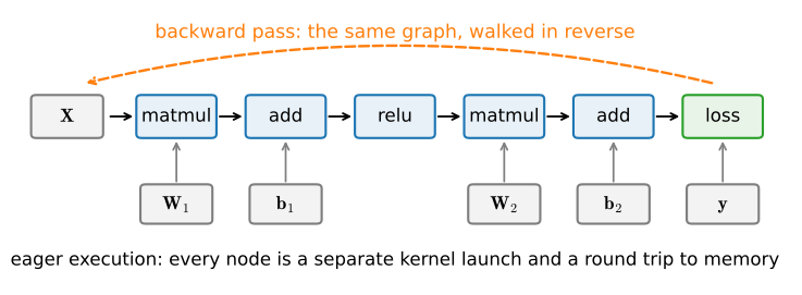
Eager execution walks this graph one node at a time, as Python reaches each line. Every node becomes a kernel launch (5–15 µs of CPU-to-GPU latency, Section 13.2) and, for a memory-bound op, a round trip to HBM. Python sees one operation, dispatches it, and moves on; it never learns that the add feeding the relu could have been done inside the same kernel. A compiler that captures the whole graph can fuse these operations before execution.
Earlier frameworks required a choice between imperative execution and symbolic graph construction. Current PyTorch and JAX workflows instead use eager execution for development and enable tracing compilation for performance. The two frameworks implement this design differently.
13.3.2 Graph Capture in PyTorch and JAX
The frameworks capture the graph in genuinely different ways, and the difference determines how each one breaks.
PyTorch — torch.compile, capture from Python bytecode. torch.compile wraps a module or function and, on first call, its front-end (TorchDynamo) inspects the Python bytecode as it runs, extracting the tensor operations into a graph while leaving the surrounding Python alone (Ansel et al. 2024). When it meets Python it cannot trace into — a data-dependent branch, a print, an unsupported library call — it does not fail; it inserts a graph break, runs that piece in ordinary Python, and resumes capturing after it (Figure 13.3.2, top). The captured pieces are compiled; the breaks are the price. It also plants guards: cheap runtime checks that the assumptions the graph was compiled under (tensor shapes, dtypes) still hold, re-compiling if they do not.
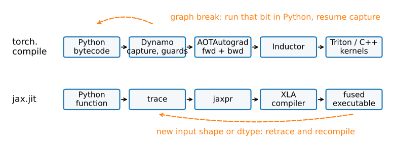
torch.compile extracts a graph from Python bytecode and falls back to Python on a graph break; jax.jit traces the function into a jaxpr and recompiles when input shapes or dtypes change.
A branch on a tensor’s value forces a graph break because the trace cannot know which path it takes until runtime:
def f(x):
    x = x * 2
    if x.sum() > 0:        # Data-dependent: forces a graph break
        return x + 1
    return x - 1

explanation = torch._dynamo.explain(f)(torch.randn(8, device=d2l.try_gpu()))
print(f'graph breaks: {explanation.graph_break_count}')
graph breaks: 1JAX — jax.jit, capture by tracing. jax.jit takes the opposite stance: it traces the function by calling it once with abstract placeholder values that record every operation they touch, producing a typed intermediate representation called a jaxpr, which XLA lowers to optimized device code (Figure 13.3.2, bottom). Tracing sees tensor operations only — anything that is not a traced array operation, like a Python print, runs once at trace time and then vanishes from the compiled function:
@jax.jit
def f(x):
    print('this prints once, at trace time')  # Not in the compiled graph
    return jnp.sin(x) + 1

x = jnp.arange(4.0)
print(jax.make_jaxpr(lambda x: jnp.sin(x) + 1)(x))  # The captured graph
_ = f(x); _ = f(x)   # Second call: no print — the trace is cached
{ lambda ; a:f32[4]. let b:f32[4] = sin a; c:f32[4] = add b 1.0:f32[] in (c,) }
this prints once, at trace timeJAX avoids graph breaks by requiring the entire function to be traceable. It cannot fall back to Python mid-graph — but in exchange it never silently splits your function into compiled fragments. Its main failure mode is recompilation: the trace is specialized to the shapes and dtypes it saw, so calling the compiled function with a new shape triggers a full retrace and recompile. In a training loop with variable-length batches this can mean recompiling every step. The escape hatches are to keep shapes static (the drop_remainder=True data-loading discipline of Section 3.2 was designed for this case), to mark genuinely constant arguments with static_argnums, and to express data-dependent control flow with lax.cond/lax.scan so it lives inside the graph rather than breaking it. The frameworks therefore require different checks: torch.compile allows more Python but must be inspected for graph breaks, whereas jax.jit requires pure traced computation and must be inspected for shape- or dtype-triggered recompilation.
13.3.3 Operation Fusion
Recall the unfused elementwise chain from Section 13.1.4 — a handful of cheap operations, each its own kernel, each a full memory round trip. Compilation fuses them into one kernel that reads the input once, does all the arithmetic in registers, and writes once:
x = torch.randn(4000, 4000, device=d2l.try_gpu())

def gelu_ish(x):
    return 0.5 * x * (1 + torch.tanh(0.8 * (x + 0.04 * x**3)))

compiled = torch.compile(gelu_ish)
# First call compiles; then verify the rewrite: same answer, then faster
assert torch.allclose(gelu_ish(x), compiled(x), atol=1e-6)

print(d2l.Benchmark(lambda: gelu_ish(x), desc='eager'))
print(d2l.Benchmark(lambda: compiled(x), desc='compiled'))
eager: 1.25 ms/call
compiled: 0.15 ms/callx = jax.random.normal(jax.random.PRNGKey(0), (4000, 4000))
def gelu_ish(x):
return 0.5 * x * (1 + jnp.tanh(0.8 * (x + 0.04 * x**3)))
compiled = jax.jit(gelu_ish)
# First call compiles; then verify the rewrite: same answer, then faster
assert jnp.allclose(gelu_ish(x), compiled(x), atol=1e-6)
print(d2l.Benchmark(lambda: gelu_ish(x), desc='eager'))
print(d2l.Benchmark(lambda: compiled(x), desc='compiled'))eager: 1.54 ms/call
compiled: 0.16 ms/callThe assert verifies that compilation preserves the result within \(10^{-6}\), allowing for floating-point reassociation. Performance is compared only after this correctness check. The fused version is close to an order of magnitude faster on this chain — and the reason is entirely on the bytes side of the roofline: the chain performs the same arithmetic either way, but eager execution makes one memory round trip per operation while the fused kernel makes a single round trip for the whole chain. Fuse eight elementwise ops and you cut roughly eight memory traversals to one. More generally, fusion exchanges kernel launches and memory traffic for arithmetic in registers. Compilation therefore helps most when Section 13.1 classifies the computation as bandwidth- or overhead-bound, and barely at all where you are already compute-bound (a single large matmul is already one well-tuned kernel; there is nothing to fuse).
When the compiler cannot fuse enough — when a memory access pattern needs restructuring, not just merging — people write the kernel by hand. The hand-written FlashAttention kernel of Section 10.5 is exactly this: the same “keep intermediates on-chip, never round-trip the big matrix” idea, executed by an expert for a pattern the general compiler cannot discover. Writing such kernels is its own craft, and it is deliberately out of scope for this book (Section 5.4 drew that fence); Triton (Tillet et al. 2019) (an important backend of torch.compile’s Inductor, which also draws on template and library kernels) and Pallas let you author them in Python-like syntax. A compiler applies many common fusion transformations automatically to the existing program.
13.3.4 Measured Training-Step Compilation
The practical application is compiling a complete training step. The two frameworks differ in which parts of that step they capture. In PyTorch, torch.compile(net) captures the model’s forward and the backward that flows through it, but the optimizer’s opt.step() below stays eager — compiling the optimizer too is possible, just not what the one-liner gives you. In JAX, nothing stops the jitted function from being the whole step: loss, gradients, and the parameter update, one compiled program. In both cases, the first call pays a fixed compilation cost, and subsequent calls have lower steady-state execution time. Whether compilation reduces total runtime depends on the number of subsequent calls:
class GeluIsh(nn.Module):  # Wraps the elementwise chain above as a layer
    def forward(self, x):
        return gelu_ish(x)

net = nn.Sequential(nn.Linear(1024, 1024), GeluIsh(),
                    nn.Linear(1024, 1024), GeluIsh(),
                    nn.Linear(1024, 1024), GeluIsh(),
                    nn.Linear(1024, 1024)).to(d2l.try_gpu())
X = torch.randn(512, 1024, device=d2l.try_gpu())
opt = torch.optim.SGD(net.parameters(), lr=0.01)

def train_step(model):
    opt.zero_grad(set_to_none=True)
    model(X).sum().backward()
    opt.step()

cnet = torch.compile(net)
t0 = time.perf_counter()
train_step(cnet); torch.cuda.synchronize()  # First call: compiles
print(f'first compiled step: {time.perf_counter() - t0:.1f} s')

print(d2l.Benchmark(lambda: train_step(net), desc='eager'))
print(d2l.Benchmark(lambda: train_step(cnet), desc='compiled'))
first compiled step: 0.3 s
eager: 2.55 ms/call
compiled: 2.05 ms/calldef loss_fn(params, X):
h = X
for W, b in params[:-1]:
h = jax.nn.gelu(h @ W + b)
W, b = params[-1]
return (h @ W + b).sum()
def train_step(params, X, lr=0.01): # Loss, gradients, AND the update
loss, grads = jax.value_and_grad(loss_fn)(params, X)
return loss, jax.tree.map(lambda p, g: p - lr * g, params, grads)
key = jax.random.PRNGKey(0)
shapes = [(1024, 1024), (1024, 1024), (1024, 1024)]
params = [(jax.random.normal(k, s) * 0.03, jnp.zeros(s[1]))
for k, s in zip(jax.random.split(key, 3), shapes)]
X = jax.random.normal(key, (512, 1024))
t0 = time.perf_counter()
compiled = jax.jit(train_step).lower(params, X).compile() # AOT: compile now
print(f'ahead-of-time compile: {time.perf_counter() - t0:.1f} s')
print(d2l.Benchmark(lambda: train_step(params, X), desc='eager'))
print(d2l.Benchmark(lambda: compiled(params, X), desc='compiled'))ahead-of-time compile: 2.5 s
eager: 21.33 ms/call
compiled: 0.21 ms/callThe compiled step is faster in steady state — a fused training step makes far fewer trips to memory and issues far fewer launches — and the first call carries a visible one-time cost while the compiler works: a fraction of a second to a couple of seconds on this toy step, depending on the framework and the state of its compile cache, and about two seconds for the real Transformer of Section 13.7. On a short experiment that price may never be repaid; on a training run of thousands of steps, the compilation cost becomes negligible per step. The JAX tab also demonstrates ahead-of-time compilation: lower(...).compile() runs the compiler as an explicit step rather than lazily on first call, returning a compiled object you can then introspect — compiled.memory_analysis() reports the memory the compiler planned before a single byte is allocated, a theme we develop in Section 13.4.
Look at the JAX ratio once more: the un-jitted step is about two orders of magnitude slower than the compiled one, because every operation in the loss, the gradient, and the update dispatches separately. JAX training steps should normally use jax.jit; un-jitted execution is useful primarily for debugging because each operation dispatches separately.
13.3.5 The Overhead Regime: Capture and Replay
Fusion reduces bandwidth costs. An overhead-bound program instead spends most of its time waiting for Python to launch small kernels and requires capture and replay. A model that is a deep stack of thin layers issues a great many small kernels, and if each takes longer to launch than to run, the device remains idle even though each kernel requires little computation (Figure 13.1.2). Compiling for fusion helps some, but the decisive fix is to stop involving Python at all: record the entire sequence of launches once, then replay it with a single command. This is what CUDA graphs do, and torch.compile exposes them through one mode flag:
# Many small layers: launch overhead dominates the actual arithmetic
deep = nn.Sequential(*[m for _ in range(60)
                       for m in (nn.Linear(256, 256), nn.Tanh())]).to(
    d2l.try_gpu())
x = torch.randn(64, 256, device=d2l.try_gpu())

reduced = torch.compile(deep, mode='reduce-overhead')
with torch.no_grad():  # Forward only: replay wants fixed buffers
    reduced(x)  # Warmup: compiles and captures the CUDA graph
    print(d2l.Benchmark(lambda: deep(x), desc='eager'))
    print(d2l.Benchmark(lambda: reduced(x), desc='reduce-overhead'))
eager: 2.25 ms/call
reduce-overhead: 0.31 ms/call# XLA already amortizes launches: the whole jitted graph is one dispatch.
deep_params = [jax.random.normal(k, (256, 256)) * 0.06
for k in jax.random.split(jax.random.PRNGKey(1), 60)]
x = jax.random.normal(jax.random.PRNGKey(2), (64, 256))
def deep_fwd(params, x):
for W in params:
x = jnp.tanh(x @ W)
return x
compiled = jax.jit(deep_fwd)
compiled(deep_params, x).block_until_ready()
print(d2l.Benchmark(lambda: deep_fwd(deep_params, x), desc='eager'))
print(d2l.Benchmark(lambda: compiled(deep_params, x), desc='jit'))eager: 9.18 ms/call
jit: 0.28 ms/callThe reduce-overhead mode captures the model’s kernel launches into a CUDA graph and replays the whole thing per call, collapsing a hundred-odd launch latencies into one. Replay is rigid: a replayed graph is a fixed sequence of kernels on fixed memory addresses, so the input shape must not change between calls (change it and PyTorch re-captures). That rigidity is also why we time the forward pass under torch.no_grad(): autograd’s saved-for-backward activations are fresh allocations on every call, and their changing addresses would force a re-capture each time. JAX needs no separate replay mechanism: a jitted function is already a single dispatched executable, so XLA amortizes launch overhead by construction — the absence of a “reduce-overhead” knob in JAX is not a missing feature but a consequence of compile-by-tracing.
13.3.6 When Compilation Hurts
Compilation is not free and not always worth it. The checklist:
- Short runs. If training lasts only a few dozen steps, compilation time may exceed the accumulated steady-state reduction. Report both first-call and repeated-call times and compute the break-even call count.
- Graph breaks in hot loops. A
torch.compiled function riddled with data-dependent branches compiles many small fragments and falls back to Python between them, keeping little of the benefit.torch._dynamo.explain(used above) counts the breaks; the fix is to remove value-dependent control flow from the hot path. - Shape churn (JAX). A
jax.jitted function called with a new shape every step recompiles every step. Pad to fixed shapes, or accept that this particular function should not be jitted. - Already compute-bound. If the profiler shows one big matmul dominating, there is nothing to fuse and no overhead to hide. Compiling is usually harmless, but measure rather than assume — compilation can also regress time or memory — and do not expect a win.
The measured performance regime determines whether compilation is appropriate. Compilation is the fix for the bandwidth and overhead regimes; reach for it when Section 13.1’s method points there, not reflexively. One last note on portability: the same capture machinery that compiles a graph can also export it — PyTorch’s torch.export emits a portable captured graph, and JAX lowers jitted functions to the StableHLO interchange format; either path lets a model run outside Python entirely, in a serving runtime or on a phone. These export paths replace earlier model-serialization mechanisms and belong to deployment rather than training.
13.3.7 Summary
- A neural network is already a compute graph (autograd builds it for the backward pass). Eager execution walks it one kernel at a time; a compiler that captures the whole graph can rewrite it — chiefly by fusing operations so intermediates stay on-chip.
torch.compilecaptures from Python bytecode and inserts graph breaks where it meets untraceable Python;jax.jittraces to a shape- specialized jaxpr with no breaks but recompiles on new shapes. Watch breaks in one, recompiles in the other.- Fusion is the fix for the bandwidth regime — close to an order of magnitude on our unfused elementwise chain — because it trades memory round trips for free register arithmetic. It barely helps already-compute-bound kernels.
torch.compile(mode="reduce-overhead")uses CUDA graphs to collapse many small launches into one replay, curing the overhead regime; XLA amortizes launches by construction and needs no such knob. Both require static shapes.- Compilation costs seconds on the first call and repays over thousands of steps. Reach for it when the method diagnoses bandwidth or overhead, not reflexively.
13.3.8 Exercises
- Introduce a data-dependent
ifinto atorch.compiled function, find the break withtorch._dynamo.explain, then rewrite the control flow withtorch.whereand confirm the break count drops to zero. What happened to the steady-state time? - Force a
jax.jitretrace by calling a jitted function with three different input lengths in a loop, and time it. Fix it by padding every input to a common length (mask the padding out of the result) and confirm the recompiles stop. Then explain whystatic_argnumsis not a fix here: a static argument becomes part of the compilation cache key, so every new value triggers a fresh trace-and-compile — verify this by putting a counter in the function and watching it tick. When isstatic_argnumsthe right tool? - Sweep the depth of the thin-layer stack from 10 to 200 at fixed width 256 and plot eager time and
reduce-overheadtime against depth. At what depth does capture-and-replay start to win, and why does the crossover exist? - Compile the matmul sweep of Section 13.1.3. For which sizes does the compiled time equal the eager time, and why? (Hint: what is a single large matmul already?)
- Time the first call and the tenth call of a compiled mid-sized training step. How many steps of steady-state savings are needed to repay the first-call compile cost? Relate the answer to the “when compilation hurts” checklist.