%matplotlib inline
from d2l import torch as d2l
import math
import torch
import numpy as np
import time2.1 Linear Regression
Suppose you are about to buy a house and want to know what a fair price is. You collect recent sales in the neighborhood, and for each one you note its area, its age, and the price it fetched. Plotting price against area, the points scatter around a rising line: bigger houses cost more, not exactly but on average. Linear regression is the tool that draws that line (and, with more than one feature, the corresponding plane or hyperplane) and turns it into a prediction for a house you have not seen.
Regression problems arise whenever we want to predict a numerical value: the price of a home or a stock, a patient’s length of stay in hospital, the demand for a product next quarter. Not every prediction is of this kind (later we turn to classification, where the target is a category rather than a number), but regression is the natural place to begin, and the running example we return to throughout this chapter is predicting house prices from area and age. In the terminology of machine learning, the dataset is called a training dataset or training set, and each row (containing the data corresponding to one sale) is called an example (or data point, instance, sample). The thing we are trying to predict (price) is called a label (or target). The variables (age and area) upon which the predictions are based are called features (or covariates).
%matplotlib inline
from d2l import tensorflow as d2l
import math
import tensorflow as tf
import numpy as np
import time%matplotlib inline
from d2l import jax as d2l
from jax import numpy as jnp
import math
import time%matplotlib inline
from d2l import mxnet as d2l
import math
from mxnet import np
import time2.1.1 Basics
Linear regression is a standard method for regression problems. Developed at the beginning of the 19th century (Legendre 1805; Gauss 1809), it begins with a small set of assumptions. First, we assume that the relationship between features \(\mathbf{x}\) and target \(y\) is approximately linear, i.e., that the conditional mean \(E[Y \mid X=\mathbf{x}]\) can be expressed as a weighted sum of the features \(\mathbf{x}\). This setup allows that the target value may still deviate from its expected value on account of observation noise. Next, we can impose the assumption that any such noise is well behaved, following a Gaussian distribution. Typically, we will use \(n\) to denote the number of examples in our dataset. We use superscripts to enumerate samples and targets, and subscripts to index coordinates. More concretely, \(\mathbf{x}^{(i)}\) denotes the \(i^{\textrm{th}}\) sample and \(x_j^{(i)}\) denotes its \(j^{\textrm{th}}\) coordinate.
2.1.1.1 Model
A model specifies how the features determine an estimate of the target. The assumption of linearity means that the expected value of the target (price) can be expressed as a weighted sum of the features (area and age):
\[\textrm{price} = w_{\textrm{area}} \cdot \textrm{area} + w_{\textrm{age}} \cdot \textrm{age} + b. \tag{2.1.1}\]
Here \(w_{\textrm{area}}\) and \(w_{\textrm{age}}\) are called weights, and \(b\) is called a bias (or offset or intercept). The weights determine the influence of each feature on our prediction. The bias determines the value of the estimate when all features are zero. Even though we will never see any newly-built homes with precisely zero area, we still need the bias because it allows us to express all linear functions of our features (rather than restricting us to lines that pass through the origin). Strictly speaking, Equation 2.1.1 is an affine transformation of input features: a linear transformation via a weighted sum, combined with a translation via the added bias. Given a dataset, our goal is to choose the weights \(\mathbf{w}\) and the bias \(b\) that, on average, make our model’s predictions fit the true prices observed in the data as closely as possible.
In disciplines that focus on datasets with just a few features, it is common to write models out long-form, as in Equation 2.1.1. In machine learning, we usually work with high-dimensional datasets, where it is more convenient to employ compact linear algebra notation. When our inputs consist of \(d\) features, we can assign each an index (between \(1\) and \(d\)) and express our prediction \(\hat{y}\) (in general the “hat” symbol denotes an estimate) as
\[\hat{y} = w_1 x_1 + \cdots + w_d x_d + b.\]
Collecting all features into a vector \(\mathbf{x} \in \mathbb{R}^d\) and all weights into a vector \(\mathbf{w} \in \mathbb{R}^d\), we can express our model compactly via the dot product between \(\mathbf{w}\) and \(\mathbf{x}\):
\[\hat{y} = \mathbf{w}^\top \mathbf{x} + b. \tag{2.1.2}\]
In Equation 2.1.2, the vector \(\mathbf{x}\) corresponds to the features of a single example. We will often find it convenient to refer to features of our entire dataset of \(n\) examples via the design matrix \(\mathbf{X} \in \mathbb{R}^{n \times d}\). Here, \(\mathbf{X}\) contains one row for every example and one column for every feature. For a collection of features \(\mathbf{X}\), the predictions \(\hat{\mathbf{y}} \in \mathbb{R}^n\) can be expressed via the matrix–vector product:
\[{\hat{\mathbf{y}}} = \mathbf{X} \mathbf{w} + b, \tag{2.1.3}\]
where broadcasting (Section 1.1.4) is applied during the summation. Given features of a training dataset \(\mathbf{X}\) and corresponding (known) labels \(\mathbf{y}\), the goal of linear regression is to find the weight vector \(\mathbf{w}\) and the bias term \(b\) such that, given features of a new data example sampled from the same distribution as \(\mathbf{X}\), the new example’s label will (in expectation) be predicted with the smallest error.
Even if we believe that the best model for predicting \(y\) given \(\mathbf{x}\) is linear, we would not expect to find a real-world dataset of \(n\) examples where \(y^{(i)}\) exactly equals \(\mathbf{w}^\top \mathbf{x}^{(i)}+b\) for all \(1 \leq i \leq n\). For example, whatever instruments we use to observe the features \(\mathbf{X}\) and labels \(\mathbf{y}\), there might be a small amount of measurement error. Thus, even when we are confident that the underlying relationship is linear, we will incorporate a noise term to account for such errors.
Before we can go about searching for the best parameters (or model parameters) \(\mathbf{w}\) and \(b\), we will need two more things: (i) a measure of the quality of some given model; and (ii) a procedure for updating the model to improve its quality.
2.1.1.2 Loss Function
Fitting the model requires a measure of prediction error. Loss functions quantify the distance between the real and predicted values of the target. The loss will usually be a nonnegative number where smaller values are better and perfect predictions incur a loss of 0. For regression problems, the most common loss function is the squared error. When our prediction for an example \(i\) is \(\hat{y}^{(i)}\) and the corresponding true label is \(y^{(i)}\), the squared error is given by:
\[l^{(i)}(\mathbf{w}, b) = \frac{1}{2} \left(\hat{y}^{(i)} - y^{(i)}\right)^2. \tag{2.1.4}\]
The constant \(\frac{1}{2}\) makes no real difference but proves to be notationally convenient, since it cancels out when we take the derivative of the loss. Note that the built-in MSE losses in most libraries omit this \(\tfrac{1}{2}\), so their gradient is twice as large; if you switch to one, halve the learning rate to compensate. Because the training dataset is given to us, and thus is out of our control, the empirical error is only a function of the model parameters. In Figure 2.1.1, we visualize the fit of a linear regression model in a problem with one-dimensional inputs.
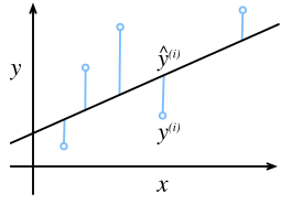
Large differences between estimates \(\hat{y}^{(i)}\) and targets \(y^{(i)}\) make disproportionately large contributions to the quadratic loss. This property strongly discourages large errors but also makes the loss sensitive to anomalous data. The following example demonstrates that sensitivity. Below we place twenty points exactly on the line \(y = 2x\), corrupt a single label, and fit a line through the origin twice: minimizing squared error (closed form) and minimizing the mean absolute error \(\frac{1}{n}\sum_i |\hat{y}^{(i)} - y^{(i)}|\) (by subgradient descent, using the subgradient \(\operatorname{sign}(\cdot)\) in place of the derivative the absolute value lacks at zero).
x = np.arange(1.0, 21.0)
y = 2 * x
y[5] = 10000                                   # corrupt a single label
w_sq = (x * y).sum() / (x * x).sum()           # closed-form squared-loss fit
w_mae = 0.0                                    # subgradient descent on MAE
for _ in range(2000):
    w_mae -= 0.002 * (np.sign(w_mae * x - y) * x).mean()
print(f'true w: 2.00, squared loss: {float(w_sq):.2f}, MAE: {float(w_mae):.2f}')
true w: 2.00, squared loss: 22.88, MAE: 2.02x = np.arange(1.0, 21.0)
y = 2 * x
y[5] = 10000 # corrupt a single label
w_sq = (x * y).sum() / (x * x).sum() # closed-form squared-loss fit
w_mae = 0.0 # subgradient descent on MAE
for _ in range(2000):
w_mae -= 0.002 * (np.sign(w_mae * x - y) * x).mean()
print(f'true w: 2.00, squared loss: {float(w_sq):.2f}, MAE: {float(w_mae):.2f}')true w: 2.00, squared loss: 22.88, MAE: 2.02x = jnp.arange(1.0, 21.0)
y = 2 * x
y = y.at[5].set(10000) # corrupt a single label
w_sq = (x * y).sum() / (x * x).sum() # closed-form squared-loss fit
w_mae = 0.0 # subgradient descent on MAE
for _ in range(2000):
w_mae -= 0.002 * (jnp.sign(w_mae * x - y) * x).mean()
print(f'true w: 2.00, squared loss: {float(w_sq):.2f}, MAE: {float(w_mae):.2f}')true w: 2.00, squared loss: 22.88, MAE: 2.02x = np.arange(1.0, 21.0)
y = 2 * x
y[5] = 10000 # corrupt a single label
w_sq = (x * y).sum() / (x * x).sum() # closed-form squared-loss fit
w_mae = 0.0 # subgradient descent on MAE
for _ in range(2000):
w_mae -= 0.002 * float((np.sign(w_mae * x - y) * x).mean())
print(f'true w: 2.00, squared loss: {float(w_sq):.2f}, MAE: {w_mae:.2f}')true w: 2.00, squared loss: 22.88, MAE: 2.02The corrupted label moves the squared-loss estimate an order of magnitude away from the generating value, while the absolute-error estimate changes little. We return to this trade-off between losses at the end of the chapter’s probabilistic treatment, and the exercises explore it further. To measure the quality of a model on the entire dataset of \(n\) examples, we average (or, up to a rescaling of the learning rate, sum) the losses on the training set:
\[L(\mathbf{w}, b) =\frac{1}{n}\sum_{i=1}^n l^{(i)}(\mathbf{w}, b) =\frac{1}{n} \sum_{i=1}^n \frac{1}{2}\left(\mathbf{w}^\top \mathbf{x}^{(i)} + b - y^{(i)}\right)^2.\]
When training the model, we seek parameters (\(\mathbf{w}^*, b^*\)) that minimize the total loss across all training examples:
\[\mathbf{w}^*, b^* = \operatorname*{argmin}_{\mathbf{w}, b}\ L(\mathbf{w}, b). \tag{2.1.5}\]
There is also a probabilistic reason for this choice. If the label equals the linear prediction plus independent Gaussian noise of constant variance, then minimizing squared error is exactly maximum-likelihood estimation. Other noise models produce other losses. We derive this correspondence and compare several choices in Section 2.1.3; for now, the squared loss supplies the objective whose optimization we study.
2.1.1.3 Analytic Solution
Unlike most of the models that we will cover, linear regression has an analytic solution for the optimal training-set parameters. We derive that solution next. First, we can subsume the bias \(b\) into the parameter \(\mathbf{w}\) by appending a column to the design matrix consisting of all 1s. Then our prediction problem is to minimize \(\|\mathbf{y} - \mathbf{X}\mathbf{w}\|^2\). The loss \(\|\mathbf{y} - \mathbf{X}\mathbf{w}\|^2\) is a convex function of \(\mathbf{w}\), so every local minimum is the global one; as long as the design matrix \(\mathbf{X}\) has full rank (no feature is linearly dependent on the others), it is strictly convex, there is just one critical point on the loss surface, and it corresponds to the minimum of the loss over the entire domain. This is why finding a single critical point suffices. Taking the derivative of the loss with respect to \(\mathbf{w}\) and setting it equal to zero yields:
\[\begin{aligned} \partial_{\mathbf{w}} \|\mathbf{y} - \mathbf{X}\mathbf{w}\|^2 = 2 \mathbf{X}^\top (\mathbf{X} \mathbf{w} - \mathbf{y}) = 0 \textrm{ and hence } \mathbf{X}^\top \mathbf{y} = \mathbf{X}^\top \mathbf{X} \mathbf{w}. \end{aligned} \tag{2.1.6}\]
If the columns of \(\mathbf{X}\) are linearly independent, solving the normal equations gives the unique minimizer
\[\mathbf{w}^* = (\mathbf X^\top \mathbf X)^{-1}\mathbf X^\top \mathbf{y} \tag{2.1.7}\]
because \(\mathbf X^\top \mathbf X\) is then invertible (Golub and Van Loan 1996). If \(\mathbf{X}\) is rank deficient, minimizers still exist but are not unique; the Moore–Penrose pseudoinverse selects the minimum-norm solution \(\mathbf{w}^*=\mathbf{X}^{\dagger}\mathbf{y}\).
The inverse formula is useful for analysis, not as a numerical recipe. Forming \(\mathbf{X}^\top\mathbf{X}\) squares the condition number, and explicitly computing an inverse adds avoidable error and work. Numerical programs should solve the least-squares problem directly with a library routine such as lstsq, which can use a QR or singular value decomposition. The mathematics appendix develops these factorizations and the pseudoinverse.
This solution has a geometric reading. As \(\mathbf{w}\) varies, the vector of predictions \(\mathbf{X}\mathbf{w}\) ranges over the column space of \(\mathbf{X}\), all linear combinations of the feature columns. Minimizing \(\|\mathbf{y}-\mathbf{X}\mathbf{w}\|^2\) therefore asks for the point in that subspace closest to the observed labels \(\mathbf{y}\), which is exactly the orthogonal projection of \(\mathbf{y}\) onto the column space. The residual \(\mathbf{y}-\mathbf{X}\mathbf{w}^*\) is what is left over, and it must be perpendicular to every feature column, precisely the statement \(\mathbf{X}^\top(\mathbf{X}\mathbf{w}^*-\mathbf{y})=\mathbf{0}\) we just derived. The same orthogonal-projection idea, for projecting onto a single direction, is developed with a picture in Section 24.1.
Some models, including linear regression with squared loss, admit analytic solutions that support direct mathematical analysis. Most deep learning models do not, so they require iterative optimization.
2.1.1.4 Minibatch Stochastic Gradient Descent
When an analytic solution is unavailable, iterative methods can still train the model effectively. Gradient descent, used throughout this book, repeatedly updates the parameters in a direction that reduces the loss locally. This algorithm is called gradient descent.
The full-batch form of gradient descent consists of taking the derivative of the loss function, which is an average of the losses computed on every single example in the dataset. For large datasets, this can be slow: we must pass over the entire dataset before making a single update, even if the update steps might be very powerful (Liu and Nocedal 1989). Redundant training examples can further reduce the benefit of computing each update from the full dataset.
The other extreme is to consider only a single example at a time and to take update steps based on one observation at a time. The resulting algorithm is stochastic gradient descent (SGD), which can be an effective strategy (Bottou 2010), even for large datasets. Single-example SGD also has computational and statistical drawbacks. One problem is that processors are a lot faster at multiplying and adding numbers than at moving data from main memory to processor cache. It is up to an order of magnitude more efficient to perform a matrix–vector multiplication than a corresponding number of vector–vector operations. This means that it can take a lot longer to process one sample at a time compared to a full batch. A second problem is that some of the layers, such as batch normalization (to be described in Section 7.3), only work well when we have access to more than one observation at a time.
The solution to both problems is to pick an intermediate strategy: rather than taking a full batch or only a single sample at a time, we take a minibatch of observations (Li et al. 2014). The specific choice of minibatch size depends on many factors, such as the amount of memory, the number of accelerators, the choice of layers, and the total dataset size. On many current accelerators, powers of \(2\) between 32 and 256 are reasonable initial candidates, but the best value depends on the task and hardware. This leads us to minibatch stochastic gradient descent.
In its most basic form, in each iteration \(t\), we first randomly sample a minibatch \(\mathcal{B}_t\) consisting of a fixed number \(|\mathcal{B}|\) of training examples. We then compute the derivative (gradient) of the average loss on the minibatch with respect to the model parameters. Finally, we multiply the gradient by a predetermined small positive value \(\eta\), called the learning rate, and subtract the resulting term from the current parameter values. We can express the update as follows:
\[(\mathbf{w},b) \leftarrow (\mathbf{w},b) - \frac{\eta}{|\mathcal{B}|} \sum_{i \in \mathcal{B}_t} \partial_{(\mathbf{w},b)} l^{(i)}(\mathbf{w},b). \tag{2.1.8}\]
In summary, minibatch SGD proceeds as follows: (i) initialize the values of the model parameters, typically at random; (ii) iteratively sample random minibatches from the data, updating the parameters in the direction of the negative gradient. For quadratic losses and affine transformations, this has a closed-form expansion:
\[\begin{aligned} \mathbf{w} & \leftarrow \mathbf{w} - \frac{\eta}{|\mathcal{B}|} \sum_{i \in \mathcal{B}_t} \partial_{\mathbf{w}} l^{(i)}(\mathbf{w}, b) && = \mathbf{w} - \frac{\eta}{|\mathcal{B}|} \sum_{i \in \mathcal{B}_t} \mathbf{x}^{(i)} \left(\mathbf{w}^\top \mathbf{x}^{(i)} + b - y^{(i)}\right)\\ b &\leftarrow b - \frac{\eta}{|\mathcal{B}|} \sum_{i \in \mathcal{B}_t} \partial_b l^{(i)}(\mathbf{w}, b) && = b - \frac{\eta}{|\mathcal{B}|} \sum_{i \in \mathcal{B}_t} \left(\mathbf{w}^\top \mathbf{x}^{(i)} + b - y^{(i)}\right). \end{aligned} \tag{2.1.9}\]
Since we pick a minibatch \(\mathcal{B}\) we need to normalize by its size \(|\mathcal{B}|\). Frequently minibatch size and learning rate are user-defined. Such tunable parameters that are not updated in the training loop are called hyperparameters. They can be tuned automatically by a number of techniques, such as Bayesian optimization (Frazier 2018). In the end, the quality of the solution is typically assessed on a separate validation dataset (or validation set).
After training for some predetermined number of iterations (or until some other stopping criterion is met), we record the estimated model parameters, denoted \(\hat{\mathbf{w}}, \hat{b}\). Note that even if our function is truly linear and noiseless, these parameters will not be the exact minimizers of the loss, nor even deterministic. Although the algorithm converges slowly towards the minimizers, it typically will not find them exactly in a finite number of steps. With a constant learning rate, minibatch SGD instead approaches a stochastic neighborhood of the minimizer whose squared radius scales like \(\eta\) times the gradient noise. Shrinking the learning rate shrinks the ball, which is why learning-rate schedules matter. Why gradient descent converges, at what rate, and how the learning rate and its schedule interact with gradient noise are worked out in Section 26.1 and Section 26.2. Moreover, we choose the minibatches \(\mathcal{B}\) at random, which breaks determinism.
Linear least squares always has a global minimizer because its loss is a convex quadratic bounded below. Full column rank, equivalently an invertible \(\mathbf{X}^\top\mathbf{X}\), makes that minimizer unique. However, the loss surfaces for deep networks contain many saddle points and minima. For prediction, we typically need parameters that leads to accurate predictions (and thus low loss). In practice, deep learning practitioners seldom struggle to find parameters that minimize the loss on training sets (Izmailov et al. 2018; Frankle and Carbin 2019). The more formidable task is to find parameters that lead to accurate predictions on previously unseen data, a challenge called generalization. We return to these topics throughout the book.
2.1.1.5 Predictions
Given the model \(\hat{\mathbf{w}}^\top \mathbf{x} + \hat{b}\), we can now make predictions for a new example, e.g., predicting the sales price of a previously unseen house given its area \(x_1\) and age \(x_2\). Deep learning practitioners often call the prediction phase inference. This is a mild misnomer: in statistics, inference more often means estimating parameters than scoring new points, so the overloaded term can confuse when the two communities talk. We will say prediction throughout.
2.1.2 Vectorization for Speed
When training our models, we typically want to process whole minibatches of examples simultaneously. Doing this efficiently requires that we vectorize the calculations and use fast linear algebra libraries rather than writing costly for-loops in Python.
To measure the effect, we compare two methods for adding vectors. To start, we instantiate two 1000-dimensional vectors containing all 1s. In the first method, we loop over the vectors with a Python for-loop. In the second, we rely on a single call to +.
n = 1000
a = d2l.ones(n)
b = d2l.ones(n)
Now we can benchmark the workloads. First, we add them, one coordinate at a time, using a for-loop.
c = d2l.zeros(n)
t = time.time()
for i in range(n):
    c[i] = a[i] + b[i]
print(f'{time.time() - t:.5f} sec')
0.02013 secc = tf.Variable(d2l.zeros(n))
t = time.time()
for i in range(n):
c[i].assign(a[i] + b[i])
print(f'{time.time() - t:.5f} sec')0.82531 sec# JAX arrays are immutable, meaning that once created their contents
# cannot be changed. For updating individual elements, JAX provides
# an indexed update syntax that returns an updated copy
c = d2l.zeros(n)
t = time.time()
for i in range(n):
c = c.at[i].set(a[i] + b[i])
print(f'{time.time() - t:.5f} sec')0.80645 secc = d2l.zeros(n)
t = time.time()
for i in range(n):
c[i] = a[i] + b[i]
print(f'{time.time() - t:.5f} sec')0.27928 secAlternatively, we rely on the overloaded + operator to compute the elementwise sum.
t = time.time()
d = a + b
print(f'{time.time() - t:.5f} sec')0.00035 sec0.00044 sec0.05211 sec0.00015 secOn this run, the second method is substantially faster than the first. The reason is not that addition itself got cheaper but that we replaced \(n\) round-trips through the Python interpreter (one per element, each dispatching a separate tensor operation) with a single call into a compiled linear-algebra kernel. The speedup therefore depends on vector length, hardware, synchronization, and framework overhead. The qualitative lesson is the same: push inner loops down into vectorized library calls rather than writing them out in Python. Moreover, we push more of the mathematics to the library so we do not have to write as many calculations ourselves, reducing the potential for errors and increasing portability of the code.
2.1.3 The Normal Distribution and Squared Loss
So far we have given a fairly functional motivation of the squared loss objective: the optimal parameters return the conditional expectation \(E[Y\mid X]\) whenever the underlying pattern is truly linear, and the loss assigns large penalties for outliers. We can also provide a more formal motivation for the squared loss objective by making probabilistic assumptions about the distribution of noise.
Linear regression and the normal distribution were both developed near the beginning of the 19th century. More importantly here, a Gaussian noise model leads directly to linear regression with squared loss.
To begin, recall that a normal distribution with mean \(\mu\) and variance \(\sigma^2\) (standard deviation \(\sigma\)) is given as
\[p(x) = \frac{1}{\sqrt{2 \pi \sigma^2}} \exp\left(-\frac{1}{2 \sigma^2} (x - \mu)^2\right).\]
Below we define a function to compute the normal distribution. We only need to plot a density, so NumPy suffices.
def normal(x, mu, sigma):
    p = 1 / math.sqrt(2 * math.pi * sigma**2)
    return p * np.exp(-0.5 * (x - mu)**2 / sigma**2)
def normal(x, mu, sigma):
p = 1 / math.sqrt(2 * math.pi * sigma**2)
return p * np.exp(-0.5 * (x - mu)**2 / sigma**2)def normal(x, mu, sigma):
p = 1 / math.sqrt(2 * math.pi * sigma**2)
return p * jnp.exp(-0.5 * (x - mu)**2 / sigma**2)def normal(x, mu, sigma):
p = 1 / math.sqrt(2 * math.pi * sigma**2)
return p * np.exp(-0.5 * (x - mu)**2 / sigma**2)We can now visualize the normal distributions.
# Use NumPy again for visualization
x = np.arange(-7, 7, 0.01)

# Mean and standard deviation pairs
params = [(0, 1), (0, 2), (3, 1)]
d2l.plot(x, [normal(x, mu, sigma) for mu, sigma in params], xlabel='x',
         ylabel='p(x)', figsize=(4.5, 2.5),
         legend=[f'mean {mu}, std {sigma}' for mu, sigma in params])
# Use NumPy again for visualization
x = np.arange(-7, 7, 0.01)

# Mean and standard deviation pairs
params = [(0, 1), (0, 2), (3, 1)]
d2l.plot(x, [normal(x, mu, sigma) for mu, sigma in params], xlabel='x',
         ylabel='p(x)', figsize=(4.5, 2.5),
         legend=[f'mean {mu}, std {sigma}' for mu, sigma in params])
# Use NumPy again for visualization
x = jnp.arange(-7, 7, 0.01)
# Mean and standard deviation pairs
params = [(0, 1), (0, 2), (3, 1)]
d2l.plot(x, [normal(x, mu, sigma) for mu, sigma in params], xlabel='x',
         ylabel='p(x)', figsize=(4.5, 2.5),
         legend=[f'mean {mu}, std {sigma}' for mu, sigma in params])
# Use NumPy again for visualization
x = np.arange(-7, 7, 0.01)

# Mean and standard deviation pairs
params = [(0, 1), (0, 2), (3, 1)]
d2l.plot(x.asnumpy(), [normal(x, mu, sigma).asnumpy() for mu, sigma in params], xlabel='x',
         ylabel='p(x)', figsize=(4.5, 2.5),
         legend=[f'mean {mu}, std {sigma}' for mu, sigma in params])
Note that changing the mean corresponds to a shift along the \(x\)-axis, and increasing the variance spreads the distribution out, lowering its peak.
One way to motivate linear regression with squared loss is to assume that observations arise from noisy measurements, where the noise \(\epsilon\) follows the normal distribution \(\mathcal{N}(0, \sigma^2)\):
\[y = \mathbf{w}^\top \mathbf{x} + b + \epsilon \textrm{ where } \epsilon \sim \mathcal{N}(0, \sigma^2). \tag{2.1.10}\]
Thus, we can now write out the likelihood of seeing a particular \(y\) for a given \(\mathbf{x}\) via
\[P(y \mid \mathbf{x}) = \frac{1}{\sqrt{2 \pi \sigma^2}} \exp\left(-\frac{1}{2 \sigma^2} (y - \mathbf{w}^\top \mathbf{x} - b)^2\right). \tag{2.1.11}\]
According to the principle of maximum likelihood, the best values of parameters \(\mathbf{w}\) and \(b\) are those that maximize the likelihood of the entire dataset:
\[P(\mathbf y \mid \mathbf X) = \prod_{i=1}^{n} p(y^{(i)} \mid \mathbf{x}^{(i)}). \tag{2.1.12}\]
The equality follows since all pairs \((\mathbf{x}^{(i)}, y^{(i)})\) were drawn independently of each other. Estimators chosen according to the principle of maximum likelihood are called maximum likelihood estimators. While maximizing the product of many exponential functions might look difficult, we can simplify things significantly, without changing the objective, by maximizing the logarithm of the likelihood instead. For historical reasons, optimizations are more often expressed as minimization rather than maximization. So, without changing anything, we can minimize the negative log-likelihood, which we can express as follows:
\[-\log P(\mathbf y \mid \mathbf X) = \sum_{i=1}^n \frac{1}{2} \log(2 \pi \sigma^2) + \frac{1}{2 \sigma^2} \left(y^{(i)} - \mathbf{w}^\top \mathbf{x}^{(i)} - b\right)^2. \tag{2.1.13}\]
If we assume that \(\sigma\) is fixed, we can ignore the first term, because it does not depend on \(\mathbf{w}\) or \(b\). The second term is identical to the squared error loss introduced earlier, except for the multiplicative constant \(\frac{1}{\sigma^2}\). The solution does not depend on \(\sigma\) either. It follows that minimizing the mean squared error is equivalent to the maximum likelihood estimation of a linear model under the assumption of additive Gaussian noise.
2.1.3.1 Selecting a Loss from a Noise Model
The same derivation applies beyond the Gaussian case. Choose a conditional model \(p(y \mid \mathbf{x})\) that represents the label noise, then minimize its negative log-likelihood. Gaussian noise yields squared error; other assumptions yield other losses:
| Output type | Noise model | Loss (negative log-likelihood) |
|---|---|---|
| real-valued, well-behaved noise | Gaussian | squared error (this section) |
| real-valued, outliers or heavy tails | Laplace | absolute error (exercise 5) |
| positive, multiplicative fluctuations (prices) | Gaussian on \(\log y\) | squared error on \(\log y\) (exercise 7) |
| counts (sales, arrivals) | Poisson | \(\lambda(\mathbf{x}) - k \log \lambda(\mathbf{x})\) (exercise 8) |
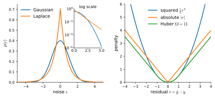
Figure 2.1.2 shows why the first two rows differ: the Laplace density places far more mass in its tails than a Gaussian of equal variance, so the Laplace model assigns a large residual more probability and its loss penalizes that residual only linearly, exactly the robustness we observed in the outlier demonstration above. The figure also marks the Huber loss, a compromise that is quadratic near zero (like squared error) but linear in the tails (like absolute error). Each of these losses is explored in the exercises; the same principle extends to heteroscedastic regression, where the noise level itself depends on the input and we predict \(\sigma(\mathbf{x})\) alongside the mean. We apply this principle again when deriving the loss for classification in the next chapter.
2.1.4 Linear Regression as a Neural Network
While linear models are not sufficiently rich to express the many complicated networks that we will introduce in this book, (artificial) neural networks are rich enough to subsume linear models as networks in which every feature is represented by an input neuron, all of which are connected directly to the output.
Figure 2.1.3 depicts linear regression as a neural network. The diagram shows the connectivity pattern, such as how each input is connected to the output, but not the specific values taken by the weights or biases.
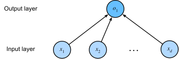
The inputs are \(x_1, \ldots, x_d\). We refer to \(d\) as the number of inputs or the feature dimensionality in the input layer. The output of the network is \(o_1\). Because we are just trying to predict a single numerical value, we have only one output neuron. Note that the input values are all given. There is just a single computed neuron. In summary, we can think of linear regression as a single-layer fully connected neural network. We will encounter networks with far more layers in later chapters.
2.1.4.1 Historical Note
The terminology of inputs, weighted connections, and activations reflects the early artificial-neuron models of McCulloch and Pitts (1943) . The analogy is limited: the affine computation above is a mathematical model, not a biological description. Modern network design is developed primarily through mathematics, statistics, computer science, and empirical study.
2.1.5 Summary
In this section, we introduced traditional linear regression, where the parameters of a linear function are chosen to minimize squared loss on the training set. We also motivated this choice of objective both via some practical considerations and through an interpretation of linear regression as maximum likelihood estimation under an assumption of linearity and Gaussian noise. After discussing both computational considerations and connections to statistics, we showed how such linear models could be expressed as simple neural networks where the inputs are directly wired to the output(s). While we will soon move past linear models altogether, they are sufficient to introduce most of the components that all of our models require: parametric forms, differentiable objectives, optimization via minibatch stochastic gradient descent, and ultimately, evaluation on previously unseen data.
2.1.6 Exercises
- Fitting a constant. Assume that we have some data \(x_1, \ldots, x_n \in \mathbb{R}\). Our goal is to find a constant \(b\) such that \(\sum_i (x_i - b)^2\) is minimized.
- Find an analytic solution for the optimal value of \(b\).
- How does this problem and its solution relate to the normal distribution?
- Change the loss to \(\sum_i |x_i-b|\). Find the optimal solution for \(b\) and describe what changes relative to the squared loss.
- Affine to linear. Prove that the affine functions that can be expressed by \(\mathbf{x}^\top \mathbf{w} + b\) are equivalent to linear functions on \((\mathbf{x}, 1)\).
- Singular design matrix. Recall that full column rank makes the linear-regression minimizer unique. Suppose instead that \(\mathbf{X}^\top \mathbf{X}\) is singular.
- Show that a minimizer still exists and characterize the set of minimizers.
- Which minimizer does the Moore–Penrose pseudoinverse select?
- How could you fix it? What happens if you add a small amount of coordinate-wise independent Gaussian noise to all entries of \(\mathbf{X}\)?
- What is the expected value of the design matrix \(\mathbf{X}^\top \mathbf{X}\) in this case?
- What happens with stochastic gradient descent when \(\mathbf{X}^\top \mathbf{X}\) does not have full rank?
- The standard remedy for a (near-)singular \(\mathbf{X}^\top \mathbf{X}\) is to add \(\lambda \mathbf{I}\) before inverting. Relate this to the \(\ell_2\) penalty introduced in Section 2.7, and show that the resulting estimator \(\mathbf{w}^* = (\mathbf{X}^\top\mathbf{X} + \lambda\mathbf{I})^{-1}\mathbf{X}^\top\mathbf{y}\) is well defined for every \(\lambda>0\).
- Laplace noise. Assume that the noise model governing the additive noise \(\epsilon\) is the Laplace distribution (see Section 27.2). That is, \(p(\epsilon) = \frac{1}{2} \exp(-|\epsilon|)\).
- Write out the negative log-likelihood of the data under the model \(-\log P(\mathbf y \mid \mathbf X)\).
- Determine whether a closed-form solution exists.
- Suggest a minibatch stochastic gradient descent algorithm to solve this problem. Identify what can go wrong near the stationary point as updates continue, and propose a fix.
- Composing two linear layers. Assume that we want to design a neural network with two layers by composing two linear layers, so that the output of the first layer becomes the input of the second layer. Explain why such a naive composition collapses to a single linear map, and state what property an intermediate operation must have to prevent the collapse.
- Beyond Gaussian noise. Suppose you use regression for realistic price estimation of houses or stock prices.
- Show that the additive Gaussian noise assumption is not appropriate. Hint: prices cannot be negative, and fluctuations scale with the price.
- Explain why regression to the logarithm of the price, i.e., \(y = \log \textrm{price}\), is much better.
- Describe what you need to worry about when dealing with pennystock, i.e., stock with very low prices. Hint: trades occur only at discrete prices, which matters more when the price is low. For more information review the celebrated Black–Scholes model for option pricing (Black and Scholes 1973).
- Counting apples. Suppose we want to use regression to estimate the number of apples sold in a grocery store.
- Identify the problems with a Gaussian additive noise model. Hint: you are selling apples, not oil.
- The Poisson distribution captures distributions over counts. It is given by \(p(k \mid \lambda) = \lambda^k e^{-\lambda}/k!\). Here \(\lambda\) is the rate function and \(k\) is the number of events you see. Prove that \(\lambda\) is the expected value of counts \(k\).
- Design a loss function associated with the Poisson distribution.
- Design a loss function for estimating \(\log \lambda\) instead.