%matplotlib inline
from d2l import torch as d2l
import gymnasium as gym
import numpy as np14.4 Temporal-Difference Learning and Exploration
Q-learning does not require a transition model or expert demonstrations. It replaces the expectation in the Bellman optimality operator with a sampled transition and updates an action-value estimate using the resulting temporal-difference error (Watkins 1989; Watkins and Dayan 1992). This substitution introduces sampling noise and makes convergence depend on which state–action pairs the behavior policy visits. We first derive and evaluate the tabular update, then study exploration through multi-armed bandits and regret.
%matplotlib inline
from d2l import jax as d2l
import gymnasium as gym
import numpy as np
14.4.1 The Sampled Backup
14.4.1.1 From the Bellman Operator to the TD Update
Value iteration, written for the action-value function, sweeps
\[Q_{k+1}(s, a) = r(s, a) + \gamma \sum_{s' \in \mathcal{S}} P(s' \mid s, a) \max_{a' \in \mathcal{A}} Q_k (s', a'); \ \textrm{for all } s \in \mathcal{S} \textrm{ and } a \in \mathcal{A}, \tag{14.4.1}\]
whose fixed point is \(Q^*\); call the right-hand side \((TQ)(s, a)\), the optimality operator of Section 14.2 on action-value tables. We use \(Q\) rather than \(V\) because extracting the optimal policy from \(Q^*\) requires only an argmax over a table row and no transition model. The kernel enters the sweep through one expectation, \(E_{s' \sim P(\cdot \mid s, a)} [\max_{a'} Q_k(s', a')]\), and an expectation can be estimated from samples. Panel (d) of Figure 14.2.1 shows this substitution: Q-learning uses one sampled successor where the exact backup sums over every successor, while retaining the maximum over next actions.
Let the agent act with some data-collection policy \(\pi_e(a \mid s)\), its behavior policy, and record \(n\) trajectories of \(T\) timesteps each, \(\{ (s_t^i, a_t^i)_{t=0,\ldots,T-1}\}_{i=1,\ldots, n}\). The Bellman equations constrain the action values of all state–action pairs. A sampled objective can impose corresponding residual terms only for pairs present in the data:
\[\hat{Q} = \mathrm{argmin}_Q \underbrace{\frac{1}{nT} \sum_{i=1}^n \sum_{t=0}^{T-1} (Q(s_t^i, a_t^i) - r(s_t^i, a_t^i) - \gamma \max_{a'} Q(s_{t+1}^i, a'))^2}_{\stackrel{\textrm{def}}{=} \ell(Q)}. \tag{14.4.2}\]
The objective does not evaluate the kernel explicitly. Instead, when the behavior policy \(\pi_e\) takes action \(a_t^i\) at state \(s_t^i\), the next state \(s_{t+1}^i\) is sampled from the transition distribution. The collected data therefore provide sampled access to the transition dynamics. For every constraint to be represented, \(\pi_e\) must keep visiting every state-action pair.
An optimal deterministic policy would not qualify: it never takes the actions it considers suboptimal, so \(\ell(Q)\) would contain no term for those state-action pairs and their values would be left unconstrained. The third part of this section takes that requirement seriously.
Instead of solving the joint problem directly, Q-learning updates individual table entries. For each observed transition \((s, a, r, s')\), it moves the corresponding entry toward the bootstrapped target \(r + \gamma \max_{a'} Q(s', a')\), treating the target as a constant even though it contains \(Q\):
\[Q(s, a) \leftarrow (1 - \alpha)\, Q(s, a) + \alpha \big( r + \gamma \max_{a'} Q(s', a') \big), \tag{14.4.3}\]
where \(\alpha\) is the step size. Because the target itself depends on \(Q\) and we deliberately hold it fixed, this is called a semi-gradient step: Q-learning is therefore not gradient descent on \(\ell(Q)\) in the strict sense; it is a semi-gradient stochastic-approximation update. Rearranged, the update is a correction proportional to a single scalar,
\[\delta = r + \gamma \max_{a'} Q(s', a') - Q(s, a), \qquad Q(s, a) \leftarrow Q(s, a) + \alpha\, \delta. \tag{14.4.4}\]
The scalar \(\delta\) is the temporal-difference error (Sutton 1988): the observed reward plus the estimated best continuation, minus the current estimate. It also appears in the actor updates of Section 15.1 and in deep Q-learning (Section 15.4).
Monte Carlo prediction waits until an episode ends and uses the realized return as a target for \(Q^{\pi_e}(s_t,a_t)\), the value of the behavior policy. The target is unbiased but contains randomness from all subsequent transitions. Temporal-difference prediction bootstraps after one step; its target is biased while the value estimate is inaccurate but usually has lower variance (Sutton 1988; Sutton and Barto 2018). Q-learning uses a maximum in this target to estimate \(Q^*\). The multi-step methods of Section 15.1 interpolate between Monte Carlo and one-step targets.
14.4.1.2 Convergence and the Double-Sampling Problem
Suppose \(\pi_e\) visits every state–action pair and collects unlimited data. Minimizing \(\ell(Q)\) then recovers the value-iteration solution when transitions are deterministic, but not in general. In the population objective, conditioning on \((s,a)\) decomposes each squared term into a squared mean and a variance:
\[L(Q) = E_{(s, a) \sim \mu} \Big[ \big( Q(s, a) - (TQ)(s, a) \big)^2 \Big] + \gamma^2\, E_{(s, a) \sim \mu} \Big[ \mathrm{Var}_{s' \sim P(\cdot \mid s, a)} \big( \max_{a'} Q(s', a') \big) \Big], \tag{14.4.5}\]
Here \(\mu\) is the visitation distribution of \(\pi_e\). The first term is the squared Bellman residual and is zero at \(Q^*\). The second term depends on \(Q\) whenever transitions are stochastic, so the minimizer of \(L\) need not be \(Q^*\). Exercise 4 gives a three-state counterexample. This is the double-sampling problem: an unbiased gradient of the squared Bellman residual requires two independent successors for the same \((s,a)\), which an ordinary environment interaction does not provide. For deterministic transitions the variance term vanishes.
Convergence instead follows from the expected update. Averaging Equation 14.4.4 over \(s'\) gives \(E[\delta\mid s,a]=(TQ)(s,a)-Q(s,a)\), which is zero at the unique fixed point \(Q^*\). Q-learning is therefore a stochastic approximation to Bellman fixed-point iteration. With the step-size conditions below and infinite visitation of every state-action pair, it converges to \(Q^*\) with probability one (Watkins and Dayan 1992; Jaakkola et al. 1994). Sampling variance affects the rate, while the behavior policy determines whether the coverage condition holds.
14.4.1.3 Step Sizes and the Robbins-Monro Conditions
For each state-action pair, the Robbins–Monro conditions are \(\sum_k\alpha_k=\infty\) and \(\sum_k\alpha_k^2<\infty\) (Robbins and Monro 1951). A constant step size violates the second condition. With stochastic transitions, its estimates continue to fluctuate around \(Q^*\). In a deterministic environment, the target has no transition noise and an update has the form \(Q(s,a)\leftarrow(1-\alpha)Q(s,a)+\alpha(TQ)(s,a)\). Updating all entries gives a contraction with modulus \((1-\alpha)+\alpha\gamma\). The sampled asynchronous method additionally requires repeated visitation of every entry.
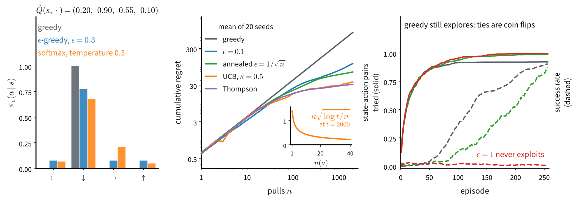
Panel (c) of Figure 14.4.1 measures this coverage for deterministic FrozenLake, where a constant step size of \(0.9\) learns quickly within the finite budget.
The conditions are necessary for the guarantee, not sufficient for a budget. The textbook sample-average rule \(\alpha = 1/(1 + n(s, a))\), with \(n(s, a)\) counting visits to the entry, passes Robbins-Monro but weights early targets computed from an inaccurate zero table as heavily as later, better-informed targets. At the tested finite budget, this slows learning substantially. Our default \(\alpha = 1/(1 + 0.1\, n(s, a))\) also passes but stays ten times larger at the same visit count. We compare all three schedules on the same seeds and report their finite-budget value errors and returns.
14.4.1.4 Terminal Masking
The update requires terminal masking in an episodic environment. When \(s'\) is terminal, its continuation value is zero, so the target contains only the immediate reward,
\[Q(s, a) \leftarrow Q(s, a) + \alpha \Big( r + \gamma\, \big(1 - \mathbf{1}(s' \textrm{ terminal})\big) \max_{a' \in \mathcal{A}} Q(s', a') - Q(s, a) \Big).\]
The mask uses terminated, not truncated: Section 14.1 distinguishes a terminal state from an observation stopped by a time limit. Treating truncation as termination would impose an incorrect zero continuation value on a nonterminal state. In code the whole repair is one factor, gamma * (1 - terminated) * Q[s_next].max().
14.4.2 Q-Learning on the Lake
14.4.2.1 The Implementation
We return to the slippery lake of Section 14.1 with the same discount. The learner accesses the environment only through reset and step; mdp, V_star, and pi_star are retained solely to compare the learned table with the exact solution.
gamma, num_episodes = 0.95, 4000
env = gym.make('FrozenLake-v1', is_slippery=True)
mdp = d2l.TabularMDP.from_gym(env, gamma)
V_star = d2l.value_iteration(mdp, num_iters=1000)[-1]
pi_star = mdp.backup(V_star).argmax(axis=1)
gamma, num_episodes = 0.95, 4000
env = gym.make('FrozenLake-v1', is_slippery=True)
mdp = d2l.TabularMDP.from_gym(env, gamma)
V_star = d2l.value_iteration(mdp, num_iters=1000)[-1]
pi_star = mdp.backup(V_star).argmax(axis=1)Two helpers, both plain numpy and both saved: the deep Q-network of Section 15.4 and the PPO of Section 15.2 will call them unchanged. The first turns a start value, an end value and a horizon into a schedule:
def linear_schedule(start, end, num_steps):
    """step -> value, interpolated from start to end, then held at end."""
    return lambda step: end + (start - end) * max(0.0, 1.0 - step / num_steps)
def linear_schedule(start, end, num_steps):
"""step -> value, interpolated from start to end, then held at end."""
return lambda step: end + (start - end) * max(0.0, 1.0 - step / num_steps)The second is the behavior policy. With probability \(\epsilon\) it takes a uniformly random action; otherwise it exploits the current table:
\[\pi_e(a \mid s) = \begin{cases} 1 - \epsilon + \epsilon/|\mathcal{A}| & a = \mathrm{argmax}_{a'} \hat{Q}(s, a') \\ \epsilon/|\mathcal{A}| & \textrm{otherwise}, \end{cases} \tag{14.4.6}\]
the \(\epsilon\)-greedy policy, with ties in the argmax broken uniformly at random. Random tie-breaking is necessary for exploration from a zero-initialized table, where every state begins as a four-way tie. In contrast, np.argmax always returns the first index:
def epsilon_greedy(q, epsilon, rng):
    """Explore with probability epsilon, else act greedily on the values q."""
    if rng.random() < epsilon:
        return int(rng.integers(len(q)))
    # Random tie-breaking is load-bearing: np.argmax would always return
    # action 0 on a zero-initialized table, and an agent that only ever
    # proposes *left* on this lake never finds the goal.
    return int(rng.choice(np.flatnonzero(q == q.max())))
def epsilon_greedy(q, epsilon, rng):
"""Explore with probability epsilon, else act greedily on the values q."""
if rng.random() < epsilon:
return int(rng.integers(len(q)))
# Random tie-breaking is load-bearing: np.argmax would always return
# action 0 on a zero-initialized table, and an agent that only ever
# proposes *left* on this lake never finds the goal.
return int(rng.choice(np.flatnonzero(q == q.max())))The implementation repeatedly selects an action, observes one transition, and changes one table entry by \(\alpha\delta\). It mutates both the value table and the visit counts; the counts determine the step-size schedule and also record state–action coverage. The exploration rate decreases from \(1\) to \(0.05\) during the first half of training and remains at that floor thereafter:
def q_learning(seed, Q, visits, env, num_episodes,
               alpha=lambda n: 1 / (1 + 0.1 * n)):
    """Tabular Q-learning; updates Q in place, yields each episode's return."""
    rng = np.random.default_rng(seed)
    epsilon = linear_schedule(1.0, 0.05, num_episodes // 2)
    env.reset(seed=seed)
    for episode in range(num_episodes):
        s, done, ret = env.reset()[0], False, 0.0
        while not done:
            a = epsilon_greedy(Q[s], epsilon(episode), rng)
            s_next, r, terminated, truncated, _ = env.step(a)
            visits[s, a] += 1
            delta = r + gamma * (1 - terminated) * Q[s_next].max() - Q[s, a]
            Q[s, a] += alpha(visits[s, a]) * delta
            s, done, ret = s_next, terminated or truncated, ret + r
        yield ret
def q_learning(seed, Q, visits, env, num_episodes,
alpha=lambda n: 1 / (1 + 0.1 * n)):
"""Tabular Q-learning; updates Q in place, yields each episode's return."""
rng = np.random.default_rng(seed)
epsilon = linear_schedule(1.0, 0.05, num_episodes // 2)
env.reset(seed=seed)
for episode in range(num_episodes):
s, done, ret = env.reset()[0], False, 0.0
while not done:
a = epsilon_greedy(Q[s], epsilon(episode), rng)
s_next, r, terminated, truncated, _ = env.step(a)
visits[s, a] += 1
delta = r + gamma * (1 - terminated) * Q[s_next].max() - Q[s, a]
Q[s, a] += alpha(visits[s, a]) * delta
s, done, ret = s_next, terminated or truncated, ret + r
yield retEvery cell here is numpy and shared between the frameworks: tabular reinforcement learning is index arithmetic, and the frameworks enter when the table becomes a network in Section 14.7. Five seeds, one plain loop:
Q = np.zeros((5, mdp.num_states, mdp.num_actions))
visits = np.zeros_like(Q)
returns = np.array([list(q_learning(k, Q[k], visits[k], env, num_episodes))
                    for k in range(5)])
d2l.plot_curves({'Q-learning': returns}, xlabel='episode',
                ylabel='return per episode', smooth=200)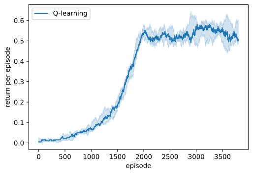
Q = np.zeros((5, mdp.num_states, mdp.num_actions))
visits = np.zeros_like(Q)
returns = np.array([list(q_learning(k, Q[k], visits[k], env, num_episodes))
                    for k in range(5)])
d2l.plot_curves({'Q-learning': returns}, xlabel='episode',
                ylabel='return per episode', smooth=200)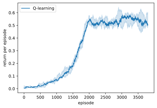
The curve is a trailing 200-episode average, with the band spanning the seeds. It remains near zero while successful episodes are rare, increases as successful transitions update preceding state–action values, and flattens after the exploration schedule reaches its floor.
14.4.2.2 The Learned Table against the Exact Solution
The curve plateaus near \(0.55\), below the optimal success probability of \(73.6\) percent measured in Section 14.2. This comparison includes failures caused by the behavior policy’s continuing exploration and therefore does not directly assess the learned table. Because the exact solution is available for this example, we can compare the learned values with \(V^*\):
print(f'max_s |V_Qhat(s) - V*(s)| per seed: '
      f'{np.round(np.abs(Q.max(axis=-1) - V_star).max(axis=-1), 3)}')
env.reset(seed=0)
opt = d2l.evaluate(env, lambda s, rng: int(pi_star[s]), num_episodes=2000)
rates = np.array([d2l.evaluate(env, lambda s, rng: int(Q[k, s].argmax()),
                               num_episodes=2000) for k in range(5)])
taxed = d2l.evaluate(env, lambda s, rng: int(pi_star[s])
                     if rng.random() > 0.05 else int(rng.integers(4)),
                     num_episodes=2000, rng=np.random.default_rng(1))
print(f'success rate: learned greedy {rates.min():.1%} to {rates.max():.1%} '
      f'over 5 seeds; pi* {opt:.1%}')
print(f'pi* forced to explore at epsilon = 0.05: {taxed:.1%}')
print(f'median environment steps: {int(np.median(visits.sum(axis=(1, 2))))}')
max_s |V_Qhat(s) - V*(s)| per seed: [0.019 0.012 0.021 0.008 0.006]
success rate: learned greedy 71.2% to 74.1% over 5 seeds; pi* 73.6%
pi* forced to explore at epsilon = 0.05: 54.1%
median environment steps: 95569print(f'max_s |V_Qhat(s) - V*(s)| per seed: '
f'{np.round(np.abs(Q.max(axis=-1) - V_star).max(axis=-1), 3)}')
env.reset(seed=0)
opt = d2l.evaluate(env, lambda s, rng: int(pi_star[s]), num_episodes=2000)
rates = np.array([d2l.evaluate(env, lambda s, rng: int(Q[k, s].argmax()),
num_episodes=2000) for k in range(5)])
taxed = d2l.evaluate(env, lambda s, rng: int(pi_star[s])
if rng.random() > 0.05 else int(rng.integers(4)),
num_episodes=2000, rng=np.random.default_rng(1))
print(f'success rate: learned greedy {rates.min():.1%} to {rates.max():.1%} '
f'over 5 seeds; pi* {opt:.1%}')
print(f'pi* forced to explore at epsilon = 0.05: {taxed:.1%}')
print(f'median environment steps: {int(np.median(visits.sum(axis=(1, 2))))}')max_s |V_Qhat(s) - V*(s)| per seed: [0.019 0.012 0.021 0.008 0.006]
success rate: learned greedy 71.2% to 74.1% over 5 seeds; pi* 73.6%
pi* forced to explore at epsilon = 0.05: 54.1%
median environment steps: 95569Across seeds, the learned value functions are within \(0.006\) to \(0.021\) of \(V^*\) in the sup norm. Their greedy policies succeed in \(71\) to \(74\) percent of evaluation episodes, compared with the optimal value of \(73.6\) percent; differences within this range are sampling error. When the optimal policy is forced to select a random action with probability \(0.05\), its success rate falls to \(54\) percent. The training curve therefore reflects both the learned policy and the continuing exploration of the behavior policy.
The median run used \(95{,}569\) environment steps. By comparison, Section 14.2 certified \(V^*\) after \(164\) sweeps of \(64\) exact model backups, or about \(10{,}500\) backups. These quantities are not directly interchangeable: a Bellman backup requires the full transition kernel, whereas an environment step provides only one sampled transition. Exercise 5 compares the two methods while keeping these different information requirements explicit.
The following panels compare the learned and exact solutions:
d2l.show_grid(env.unwrapped.desc, np.stack([Q[0].max(-1), V_star]),
              np.stack([Q[0].argmax(-1), pi_star]),
              titles=['Q-learning, seed 0', 'value iteration'])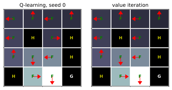
d2l.show_grid(env.unwrapped.desc, np.stack([Q[0].max(-1), V_star]),
              np.stack([Q[0].argmax(-1), pi_star]),
              titles=['Q-learning, seed 0', 'value iteration'])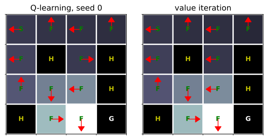
The learned arrows reproduce the slip-aware strategy of Section 14.2 except at state \(6\): Q-learning selects right, whereas \(\pi^*\) selects left. State \(6\) lies between holes \(5\) and \(7\), and the two actions have equal values under \(Q^*\), so this disagreement is a different resolution of an exact tie. The value estimates are most accurate in frequently visited states and coarser in the rarely visited top-right corner.
Now consider the deterministic special case. Disabling slip produces deterministic transitions and noiseless targets, for which the damped-contraction argument permits the constant \(\alpha = 0.9\). In this experiment, one sixteenth of the episode budget suffices:
calm = gym.make('FrozenLake-v1', is_slippery=False)
table = np.zeros((mdp.num_states, mdp.num_actions))
for _ in q_learning(0, table, np.zeros_like(table), calm, 256,
                    alpha=lambda n: 0.9):
    pass
print(f'calm ice, 256 episodes, alpha = 0.9: greedy policy succeeds '
      f'{d2l.evaluate(calm, lambda s, rng: int(table[s].argmax()), 100):.0%}')
calm ice, 256 episodes, alpha = 0.9: greedy policy succeeds 100%calm = gym.make('FrozenLake-v1', is_slippery=False)
table = np.zeros((mdp.num_states, mdp.num_actions))
for _ in q_learning(0, table, np.zeros_like(table), calm, 256,
alpha=lambda n: 0.9):
pass
print(f'calm ice, 256 episodes, alpha = 0.9: greedy policy succeeds '
f'{d2l.evaluate(calm, lambda s, rng: int(table[s].argmax()), 100):.0%}')calm ice, 256 episodes, alpha = 0.9: greedy policy succeeds 100%In the deterministic environment, the same method finds a perfect policy with about one sixteenth as many episodes and can use a much larger step size. This contrast shows how transition noise changes the sample and step-size requirements. To compare the three schedules, we track \(Q(s_0,\textrm{left})\) across the same five seeds; its exact value is available from dynamic programming.
Q_star = mdp.backup(V_star)
a0 = int(pi_star[0])
print(f'Q*(s0, {"<v>^"[a0]}) = {Q_star[0, a0]:.3f}')
trace = {}
for name, alpha in [('0.9 (constant)', lambda n: 0.9),
                    ('1/(1 + 0.1 n)', lambda n: 1 / (1 + 0.1 * n)),
                    ('1/(1 + n)', lambda n: 1 / (1 + n))]:
    runs = []
    for seed in range(5):
        Qa = np.zeros_like(Q[0])
        runs.append([Qa[0, a0] for _ in q_learning(
            seed, Qa, np.zeros_like(Qa), env, num_episodes, alpha)])
    trace[f'alpha = {name}'] = np.array(runs)
    print(f'alpha = {name:>14}: final estimates {np.round(runs, 3)[:, -1]}')
d2l.plot_curves(trace, xlabel='episode', ylabel='estimate of Q(s0, left)',
                reference=Q_star[0, a0])
Q*(s0, <) = 0.180
alpha = 0.9 (constant): final estimates [0.056 0.221 0.206 0.265 0.236]
alpha = 1/(1 + 0.1 n): final estimates [0.19 0.186 0.195 0.184 0.18 ]
alpha = 1/(1 + n): final estimates [0.003 0.024 0.008 0.009 0.002]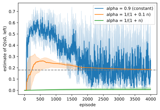
Q_star = mdp.backup(V_star)
a0 = int(pi_star[0])
print(f'Q*(s0, {"<v>^"[a0]}) = {Q_star[0, a0]:.3f}')
trace = {}
for name, alpha in [('0.9 (constant)', lambda n: 0.9),
                    ('1/(1 + 0.1 n)', lambda n: 1 / (1 + 0.1 * n)),
                    ('1/(1 + n)', lambda n: 1 / (1 + n))]:
    runs = []
    for seed in range(5):
        Qa = np.zeros_like(Q[0])
        runs.append([Qa[0, a0] for _ in q_learning(
            seed, Qa, np.zeros_like(Qa), env, num_episodes, alpha)])
    trace[f'alpha = {name}'] = np.array(runs)
    print(f'alpha = {name:>14}: final estimates {np.round(runs, 3)[:, -1]}')
d2l.plot_curves(trace, xlabel='episode', ylabel='estimate of Q(s0, left)',
                reference=Q_star[0, a0])
Q*(s0, <) = 0.180
alpha = 0.9 (constant): final estimates [0.056 0.221 0.206 0.265 0.236]
alpha = 1/(1 + 0.1 n): final estimates [0.19 0.186 0.195 0.184 0.18 ]
alpha = 1/(1 + n): final estimates [0.003 0.024 0.008 0.009 0.002]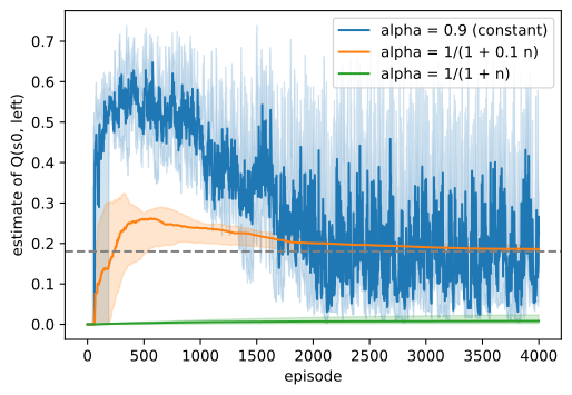
The constant step size does not converge to a fixed value: after four thousand episodes, the five estimates range from \(0.06\) to \(0.27\), compared with the exact value \(0.180\). The default decreasing schedule places all five estimates between \(0.180\) and \(0.195\). The sample-average schedule \(1/(1+n)\) also satisfies the Robbins–Monro conditions, but all five estimates remain below \(0.025\) at this budget because early, inaccurate targets retain substantial weight. The asymptotic conditions therefore do not determine which schedule performs best at a finite horizon.
14.4.2.3 Feedback between Estimation and Data Collection
The behavior policy depends on the current value estimates, so estimation errors influence which data are collected next. If \(\hat{Q}(s,a)\) is too large, an \(\epsilon\)-greedy policy selects \(a\) more often and produces additional transitions whose expected TD errors reduce the overestimate. An underestimate is corrected less directly, because the action may be selected only through random exploration. This creates an asymmetry between overestimation and underestimation.
At a fixed point, the expected correction must vanish for every state–action pair visited by the behavior policy. By Equation 14.4.4, this is precisely the Bellman optimality condition on the visited set. Interaction can therefore direct data collection toward errors in the current estimate. Offline reinforcement learning, introduced in Section 15.6, removes this feedback because it learns from a fixed dataset.
The preceding argument assumes continued exploration. To isolate the resulting tradeoff, we next study a multi-armed bandit, which removes state transitions and delayed rewards.
14.4.3 Exploration and Regret
14.4.3.1 The Multi-Armed Bandit
To isolate exploration, use the one-state MDP from Section 14.1. Without transitions or delayed rewards, the resulting multi-armed bandit requires the agent to balance estimating action values against selecting actions with high expected reward. We use ten Bernoulli arms, one of which has the largest success probability:
arms = np.array([0.50, 0.42, 0.90, 0.25, 0.55, 0.38, 0.60, 0.32, 0.50, 0.45])

def bandit_run(rule, num_pulls, seed):
    """One state, one step: pull an arm, log the shortfall, update tallies."""
    rng = np.random.default_rng(seed)
    wins, count = np.zeros(len(arms)), np.zeros(len(arms))
    gap = np.empty(num_pulls)
    for t in range(num_pulls):
        a = rule(wins, count, t, rng)
        count[a] += 1
        wins[a] += float(rng.random() < arms[a])
        gap[t] = arms.max() - arms[a]
    return np.cumsum(gap)
arms = np.array([0.50, 0.42, 0.90, 0.25, 0.55, 0.38, 0.60, 0.32, 0.50, 0.45])
def bandit_run(rule, num_pulls, seed):
"""One state, one step: pull an arm, log the shortfall, update tallies."""
rng = np.random.default_rng(seed)
wins, count = np.zeros(len(arms)), np.zeros(len(arms))
gap = np.empty(num_pulls)
for t in range(num_pulls):
a = rule(wins, count, t, rng)
count[a] += 1
wins[a] += float(rng.random() < arms[a])
gap[t] = arms.max() - arms[a]
return np.cumsum(gap)A bandit policy is any rule from the running tallies to an arm, so epsilon_greedy applies unchanged to the empirical means. In a contextual bandit, a fresh context arrives each round independently of previous actions, one action is scored, and the episode ends. The model may generalize across contexts, but there are no controlled dynamics or delayed rewards. Section 15.7 uses this distinction when classifying single-turn preference optimization.
14.4.3.2 Regret and the Epsilon-Greedy Family
A bandit permits evaluation by cumulative regret rather than success rate. Each pull contributes the gap between the best mean \(\mu^* = \max_a \mu_a\) and the selected arm’s mean,
\[\textrm{regret after } t \textrm{ pulls} = \sum_{u=1}^{t} \big( \mu^* - \mu_{a_u} \big),\]
which is what bandit_run accumulates. Its expectation is \(\sum_a (\mu^* - \mu_a)\, E[n(a)]\): the gap of each arm multiplied by its expected number of pulls. Sublinear regret means that average regret per pull converges to zero. We compare three members of the \(\epsilon\)-greedy family over twenty independent runs:
def eps_rule(schedule):
    """Epsilon-greedy on the empirical means, with epsilon = schedule(t)."""
    return lambda wins, count, t, rng: epsilon_greedy(
        wins / np.maximum(count, 1), schedule(t), rng)

rules = {'greedy': eps_rule(lambda t: 0.0),
         'epsilon = 0.1': eps_rule(lambda t: 0.1),
         'annealed': eps_rule(lambda t: max(0.02, 1 / np.sqrt(t + 1)))}
regret = {name: np.array([bandit_run(rule, 2000, [2026, i, s])
                          for s in range(20)])
          for i, (name, rule) in enumerate(rules.items())}
for name, r in regret.items():
    print(f'{name:>13}: mean regret after 2000 pulls {r[:, -1].mean():6.1f}')
greedy: mean regret after 2000 pulls 824.0
epsilon = 0.1: mean regret after 2000 pulls 116.5
annealed: mean regret after 2000 pulls 68.5def eps_rule(schedule):
"""Epsilon-greedy on the empirical means, with epsilon = schedule(t)."""
return lambda wins, count, t, rng: epsilon_greedy(
wins / np.maximum(count, 1), schedule(t), rng)
rules = {'greedy': eps_rule(lambda t: 0.0),
'epsilon = 0.1': eps_rule(lambda t: 0.1),
'annealed': eps_rule(lambda t: max(0.02, 1 / np.sqrt(t + 1)))}
regret = {name: np.array([bandit_run(rule, 2000, [2026, i, s])
for s in range(20)])
for i, (name, rule) in enumerate(rules.items())}
for name, r in regret.items():
print(f'{name:>13}: mean regret after 2000 pulls {r[:, -1].mean():6.1f}') greedy: mean regret after 2000 pulls 824.0
epsilon = 0.1: mean regret after 2000 pulls 116.5
annealed: mean regret after 2000 pulls 68.5The greedy rule is sensitive to its first observations. It incurs little subsequent regret if it identifies the best arm early, but it can remain committed to a suboptimal arm; its mean regret is \(824\). With fixed \(\epsilon = 0.1\), the best arm is usually identified quickly, but uniform exploration continues throughout the run. For these arms this produces approximately \(0.04\) regret per pull and a total of \(117\). Annealing \(\epsilon\) reduces exploration as the estimates improve and lowers the total regret to \(69\).
14.4.3.3 Optimism: UCB and Thompson Sampling
Panel (a) of Figure 14.4.1 represents the preceding policies as distributions over a row of action values. It also includes the softmax policy introduced in Section 14.5, whose temperature controls how concentrated the distribution is. The two remaining methods use uncertainty to direct exploration. Optimistic initialization starts each estimate above the attainable rewards, so an arm continues to be selected until observations lower its estimate (Sutton and Barto 2018). The upper confidence bound (UCB) rule instead adds an uncertainty bonus and selects the largest upper confidence estimate:
\[a_t = \underset{a}{\mathrm{argmax}} \Big[ \hat{\mu}(a) + \kappa \sqrt{\log t \,/\, n(a)} \Big], \tag{14.4.7}\]
The bonus decreases with the number of observations \(n(a)\) and increases slowly with \(t\) while an arm is not selected (Auer et al. 2002). Thus UCB adapts exploration separately for each arm. With the standard coefficient \(\kappa=\sqrt{2}\), its regret is logarithmic in \(t\), whereas fixed-\(\epsilon\) exploration has linear regret. Smaller coefficients can work better on a particular finite problem but no longer satisfy that guarantee. Each arm is played once to initialize its index; subsequent choices are deterministic maximizers of the UCB score. Thompson sampling (Thompson 1933) takes a Bayesian approach. For Bernoulli rewards it maintains a Beta posterior for each arm, samples one mean from each posterior, and selects the arm with the largest sample. As observations accumulate, both methods concentrate their choices on well-supported arms:
kappa = 0.5

def ucb(wins, count, t, rng):
    if (count == 0).any():          # play each arm once before pricing any
        return int(np.argmax(count == 0))
    return int(np.argmax(wins / count + kappa * np.sqrt(np.log(t) / count)))

def thompson(wins, count, t, rng):
    return int(rng.beta(1 + wins, 1 + count - wins).argmax())

for i, (name, rule) in enumerate([('UCB', ucb), ('Thompson', thompson)], 3):
    regret[name] = np.array([bandit_run(rule, 2000, [2026, i, s])
                             for s in range(20)])
    print(f'{name:>13}: mean regret after 2000 pulls '
          f'{regret[name][:, -1].mean():6.1f}')
d2l.plot_curves(regret, xlabel='pulls', ylabel='cumulative regret')
UCB: mean regret after 2000 pulls 36.5
Thompson: mean regret after 2000 pulls 31.5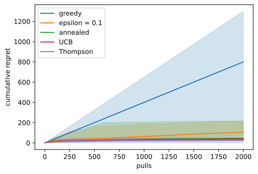
kappa = 0.5

def ucb(wins, count, t, rng):
    if (count == 0).any():          # play each arm once before pricing any
        return int(np.argmax(count == 0))
    return int(np.argmax(wins / count + kappa * np.sqrt(np.log(t) / count)))

def thompson(wins, count, t, rng):
    return int(rng.beta(1 + wins, 1 + count - wins).argmax())

for i, (name, rule) in enumerate([('UCB', ucb), ('Thompson', thompson)], 3):
    regret[name] = np.array([bandit_run(rule, 2000, [2026, i, s])
                             for s in range(20)])
    print(f'{name:>13}: mean regret after 2000 pulls '
          f'{regret[name][:, -1].mean():6.1f}')
d2l.plot_curves(regret, xlabel='pulls', ylabel='cumulative regret')
UCB: mean regret after 2000 pulls 36.5
Thompson: mean regret after 2000 pulls 31.5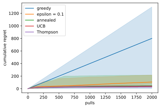
Both methods have lower regret than the \(\epsilon\)-greedy variants in this experiment. The curvature on the logarithmic plot is consistent with logarithmic regret, but \(2000\) pulls cannot verify an asymptotic rate. The coefficient also matters: \(\kappa=0.5\) was selected for these arms; \(\kappa=\sqrt{2}\) gives regret near \(200\), while \(\kappa=0.15\) sometimes commits to a suboptimal arm and in one of twenty runs exceeds \(900\). At \(\kappa=0.5\), total regret ranges from \(21\) to \(53\) across seeds. The relative performance of UCB and Thompson sampling is therefore specific to this experiment.
Online and offline uncertainty. UCB adds an uncertainty term because an online agent can test optimistic estimates by collecting new observations. Offline methods often subtract an uncertainty penalty because no new data can correct an overestimate (Section 15.6). The two terms express a related principle, but they are calibrated differently. UCB uses the online count and time, whereas an offline penalty is defined relative to a fixed dataset.
14.4.3.4 Exploration in MDPs
Bandit actions are immediately available, whereas an uncertain state-action pair in an MDP may be reachable only through a particular sequence of actions. Under independent random exploration, the probability of executing a required sequence of \(k\) actions decreases geometrically with \(k\). Difficult MDPs therefore require exploration over temporally extended behavior.
One approach assigns bonuses to uncertain state-action pairs and propagates them through value backups, so the policy selects action sequences leading toward uncertain states. With function approximation, explicit counts are unavailable; alternatives include density-model pseudo-counts, curiosity based on prediction error, random network distillation, state archives, and ensembles for approximate posterior sampling (Burda et al. 2019). FrozenLake does not expose this difficulty. With only 44 nonterminal state–action pairs, the exploration schedules used here provide broad coverage within the training budget.
14.4.4 Off-Policy Learning
14.4.4.1 The Off-Policy Mechanism
The \(\max_{a'}\) in Equation 14.4.4 evaluates a greedy continuation independently of the action that the behavior policy actually takes at \(s'\). Q-learning is therefore off-policy: it estimates the value of the greedy policy while data are generated by the exploratory policy \(\pi_e\). SARSA is the corresponding on-policy method; it bootstraps from the next action actually selected and estimates the value of the behavior policy, including its exploration (Sutton and Barto 2018). This distinction explains why Q-learning can use persistent exploration while its reported greedy policy agrees with \(\pi^*\). It also permits learning from older experience, another agent, or a fixed log, provided the data continue to cover the state–action pairs required by the target policy. Function approximation can make this flexibility unstable (Section 15.4), and a fixed dataset imposes the stronger coverage constraints studied in Section 15.6.
14.4.4.2 Maximization Bias
The maximum of noisy estimates tends to exceed the maximum of their expectations because it selects entries with positive estimation errors. This produces maximization bias in bootstrapped targets. In the experiment, four of five final estimates of \(Q(s_0,\textrm{left})\) exceed the true value \(0.180\), and the fifth agrees to the reported precision. The bias decreases as tabular estimates converge, but it can persist under function approximation. Double Q-learning reduces it by using separate estimators to select and evaluate the maximizing action, although the resulting estimates can also be low (Hasselt 2010). Section 15.4 studies this method.
14.4.5 Summary
Q-learning replaces the expectation in a Bellman backup with a sampled transition. Its temporal-difference update is \(Q \leftarrow Q + \alpha \delta\). In stochastic environments, this semi-gradient update should not be confused with minimizing a sampled squared Bellman residual, whose population objective contains an additional variance term. Under sustained visitation and Robbins–Monro step sizes, tabular Q-learning converges to \(Q^*\). Exploration can be studied separately in a one-state bandit: fixed-\(\epsilon\) exploration has linear regret, whereas UCB and Thompson sampling reduce exploration as uncertainty decreases. The maximum in the target makes Q-learning off-policy and also introduces maximization bias.
Replacing the table by a neural network gives the deep Q-learning methods developed in Section 15.4.
Experimental scope. The FrozenLake results use five seeds, one finite state space, and a fixed training budget. They show that tabular Q-learning approaches the exact solution under the tested schedule, but they do not establish an optimal schedule or a scaling law. The bandit curves average twenty runs; the UCB coefficient was tuned for these arms, and \(2{,}000\) pulls are insufficient to verify an asymptotic regret rate. The reported exploration cost is specific to the geometry of this environment.
14.4.6 Exercises
- [conceptual] Why greedy from the start cannot work. On a zero table every state is a four-way tie. Suppose
epsilon_greedyalways returned action \(0\) (left) instead of breaking ties at random: describe the resulting trajectory and what the algorithm would report after any number of episodes. With random tie-breaking but \(\epsilon = 0\) throughout, what does panel (c) of Figure 14.4.1 show about coverage, and why does coverage alone not guarantee a good table? - [short-code] The exploration schedule. Predict, then measure. Modify
q_learningto accept the \(\epsilon\) schedule as an argument, and run with \(\epsilon\) held at \(0\), \(0.1\), \(0.5\) and \(1\), and with the annealed schedule. For each, report the episode of the first success andd2l.evaluateof the final greedy policy over \(1000\) episodes. Which setting wins on each number, and why is the training return alone a misleading basis for choosing? - [conceptual] Step sizes under a finite budget. Which of the three schedules of the section’s step-size cell satisfy the Robbins-Monro conditions \(\sum_k \alpha_k = \infty\) and \(\sum_k \alpha_k^2 < \infty\)? Explain why the constant step is nevertheless sound on the calm map (write the noiseless update as \(Q \leftarrow (1 - \alpha) Q + \alpha\, TQ\) and compute its contraction modulus) and why it cannot settle on ice. Explain the stranding of \(1/(1 + n)\) in one sentence about how a sample average weights early targets, then find by experiment a \(c\) for which \(\alpha = 1/(1 + c\, n)\) beats both decaying schedules at the same budget.
- [short-code] The double-sampling counterexample. Build the three-state MDP: from state \(s\) a single action gives reward \(0\) and moves to \(u_1\) or \(u_2\) with probability \(1/2\) each; from \(u_1\) a single action gives reward \(1\) and terminates; from \(u_2\), \(0\) and terminates. (i) Write down \(Q^*\) for all three pairs. (ii) With \(\mu\) uniform over the pairs, write the population objective Equation 14.4.5 explicitly and minimize it, in closed form or over a grid: at \(\gamma = 0.95\) the minimizer assigns roughly \(0.845\) and \(0.155\) to the two successor pairs whose true values are \(1\) and \(0\). (iii) Verify that the semi-gradient update Equation 14.4.4, with each pair visited equally often and a decaying step, converges to \(Q^*\) instead. What extra data access would make the argmin of Equation 14.4.2 unbiased, and why does the name double sampling fit?
- [short-code] A like-for-like comparison with value iteration. Take \(Q^*\) as ground truth. Plot \(\|\hat{Q} - Q^*\|_\infty\) for Q-learning against environment steps (the
visitsledger counts them), and for value iteration, $Q_k = $mdp.backupof \(V_k\), against Bellman backups at \(64\) per sweep. Which comparison is fair under which assumption, and what resource does each algorithm use? - [short-code] Regret, measured properly. Means over \(20\) runs can hide tails: re-plot the five rules’ cumulative regret on doubly logarithmic axes, per seed rather than averaged. Which rules are sublinear, and which show heavy tails? Then rerun UCB at \(\kappa \in \{0.15, 0.3, 0.5, 1.2, 2.4\}\) and at the theorem’s \(\sqrt{2}\): how sensitive is the mean regret, which failure lives at each end (too small turns the rule greedy and revives the heavy tail; too large causes excessive exploration), and where does UCB fall behind the annealed schedule? Summarize in one sentence what UCB tunes that \(\epsilon\)-greedy does not.
- [extended] A harder map. Move to the \(8 \times 8\) map,
gym.make('FrozenLake-v1', map_name='8x8', is_slippery=True), with the section’s code unchanged. With the section’s budget the agent may never see the goal at all: report, over ten seeds, how many episodes of uniform random behavior pass before the first success, and reconcile the number with a random-walk hitting-time estimate. Then find a schedule and budget that reliably solve the map, and report the cost in environment steps next to the section’s \(4 \times 4\) figure. (Budget about five minutes.)